install.packages("mapSpain", dependencies = TRUE)Welcome to mapSpain
Motivation
mapSpain provides political and administrative boundaries of Spain at several levels. It also supports static map tiles from WMS and WMTS services, either as georeferenced rasters for static maps or as layers in interactive leaflet maps.
The package also includes helpers to translate and convert Spanish subdivision names and codes. These helpers make it easier to join, clean and transform data, whether or not the data is spatial.
The main data sources used by mapSpain are:
- GISCO (Eurostat), through the giscoR package.
- CartoBase ANE (Atlas Nacional de España), provided by the Instituto Geográfico Nacional (IGN).
- Spanish public institutions that publish WMTS and WMS tile services (https://www.idee.es/web/idee/segun-tipo-de-servicio).
Most functions return sf objects or SpatRaster objects from the terra package.
Package website: https://ropenspain.github.io/mapSpain/.
Installation
CRAN
Development version
Use r-universe:
# Enable this universe.
install.packages(
  "mapSpain",
  repos = c(
    "https://ropenspain.r-universe.dev",
    "https://cloud.r-project.org"
  ),
  dependencies = TRUE
)
Installation with pak from GitHub
install.packages("pak")
pak::pak("rOpenSpain/mapSpain", dependencies = TRUE)
A quick example
library(mapSpain)
library(tidyverse)

galicia <- esp_get_munic_siane(
  region = "Galicia",
  cache_dir = "./maps_spain/"
) |>
  # Standardize labels.
  mutate(Provincia = esp_dict_translate(ine.prov.name, "es"))

ggplot(galicia) +
  geom_sf(aes(fill = Provincia), color = "grey70") +
  labs(title = "Provinces of Galicia") +
  scale_fill_discrete(type = hcl.colors(4, "Blues")) +
  theme_bw()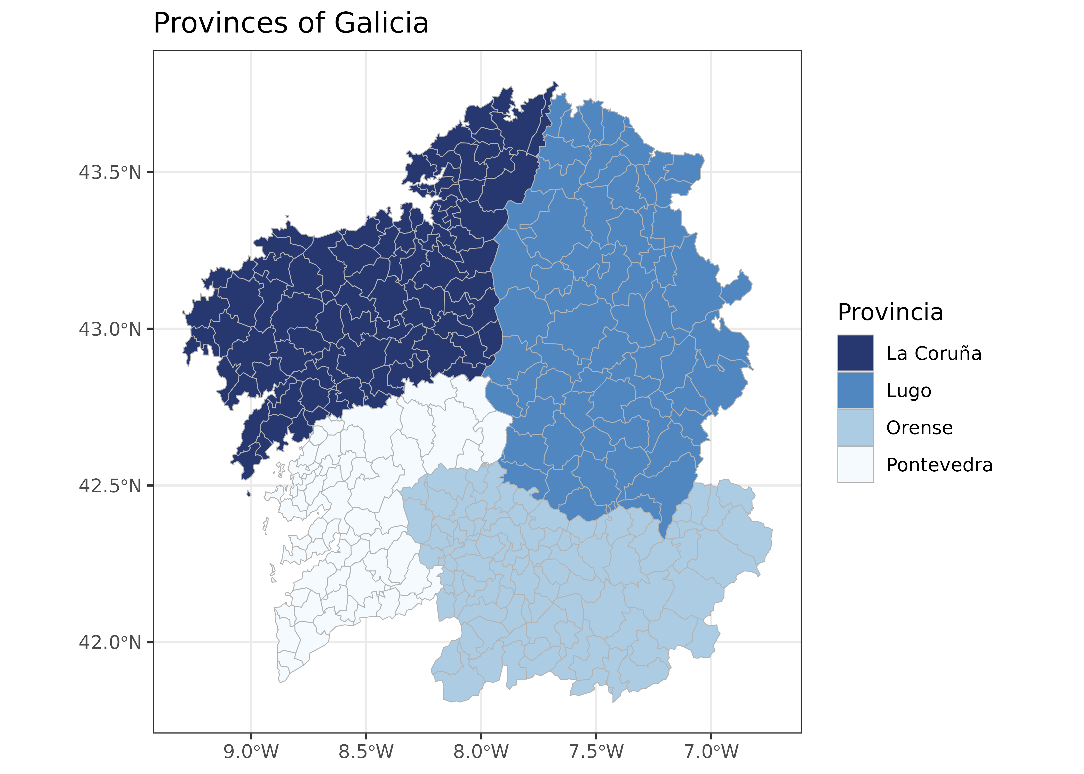
You can also inspect the dataset interactively:
Comparing mapSpain with other packages
The following example compares mapSpain with packages that provide sf or SpatVector country boundaries.
library(sf) # Spatial data manipulation.

# rnaturalearth
library(rnaturalearth)
esp_rnat <- ne_countries("large", country = "Spain", returnclass = "sf") |>
  st_transform(3857)

# mapSpain.
esp_mapspain <- esp_get_spain(epsg = 4326) |>
  st_transform(3857)

# geodata (GADM)
library(geodata)
esp_geodata <- geodata::gadm("ES",
  path = "./maps_spain/", level = 0
) |>
  # Convert from SpatVector to an sf object.
  sf::st_as_sf() |>
  st_transform(3857)

# geobounds
library(geobounds)
esp_geobounds <- geobounds::gb_get_adm0("ESP",
  cache_dir = "./maps_spain/"
) |>
  st_transform(3857)

# Orthophoto of the Ferrol estuary.
tile <- esp_get_munic_siane(
  munic = "Ferrol", epsg = 3857,
  cache_dir = "./maps_spain/"
) |>
  esp_get_tiles("PNOA",
    bbox_expand = 0.5, zoommin = 1,
    cache_dir = "./maps_spain/"
  )

# Prepare the plot.
library(tidyterra)

esp_all <- bind_rows(esp_rnat, esp_mapspain, esp_geodata, esp_geobounds)

esp_all$source <- as_factor(c(
  "rnaturalearth",
  "mapSpain",
  "geodata (GADM)",
  "geoBoundaries"
))

ggplot(esp_all) +
  geom_spatraster_rgb(data = tile, maxcell = Inf, alpha = 0.5) +
  geom_sf(
    aes(color = source, linetype = source),
    fill = NA,
    show.legend = "line",
    linewidth = 0.5,
    alpha = 0.7
  ) +
  coord_sf(
    crs = 4326,
    xlim = c(-8.384421, -8.154413),
    ylim = c(43.43201, 43.59545),
    expand = FALSE
  ) +
  scale_color_manual(values = c("red", "black", "blue", "orange")) +
  scale_linetype_manual(values = c("solid", "dotted", "dashed", "twodash")) +
  theme_void() +
  labs(title = "Ferrol estuary")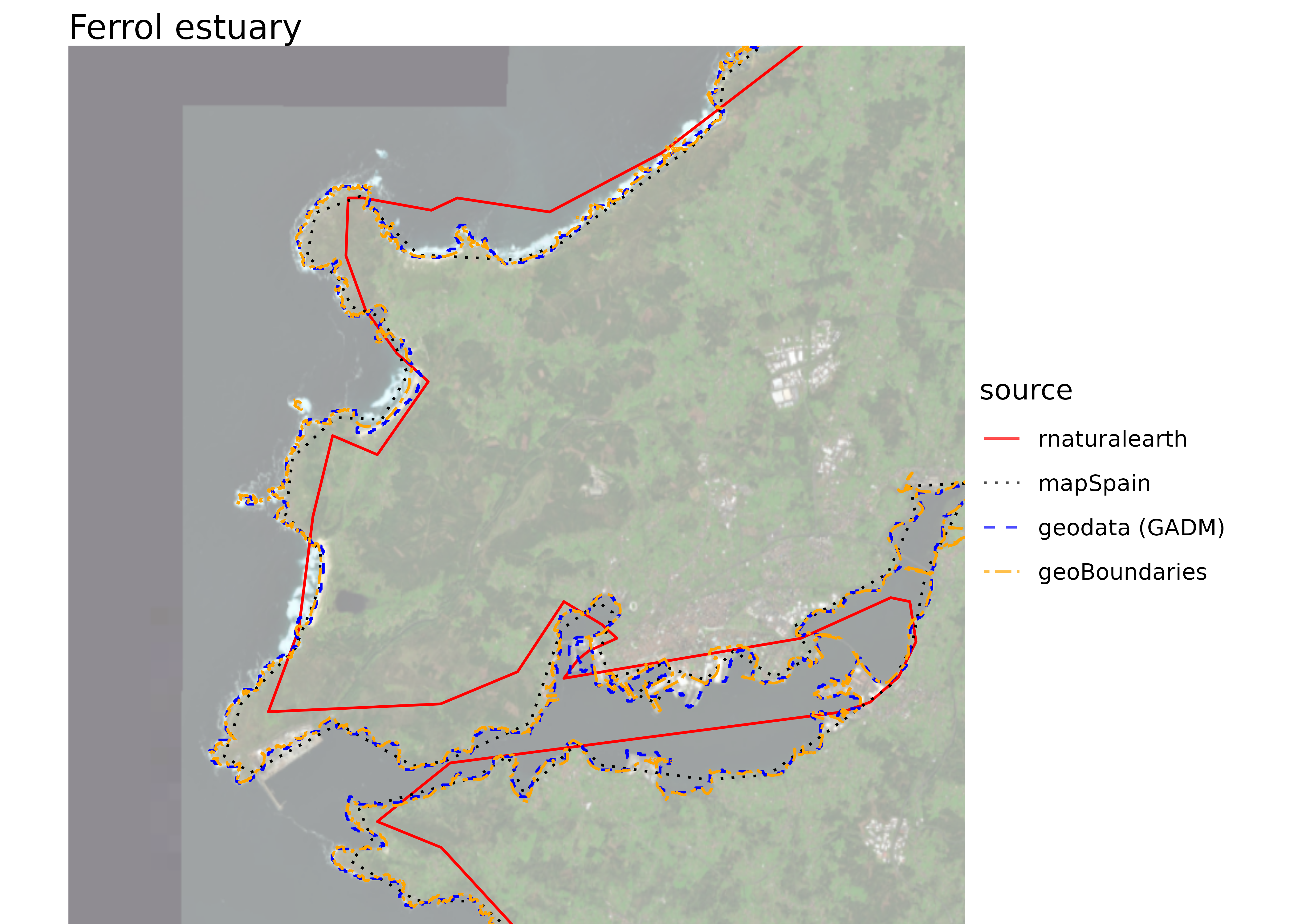
- rnaturalearth: lower boundary precision.
- mapSpain: good boundary precision for this use case.
- GADM (through geodata): very high boundary precision.
- geoBoundaries (through geobounds): good boundary precision for this use case.
Caching
mapSpain uses web resources. By default, downloaded files are stored in tempdir() for reuse during the current session.
Use esp_set_cache_dir() to choose a user-specific download directory. Add install = TRUE to make that cache configuration persistent across sessions.
esp_set_cache_dir("~/R/mapslib/mapSpain", install = TRUE, verbose = TRUE)

#> ℹ mapSpain cache directory is C:/Users/XXXX/Documents/R/mapslib/mapSpain.

munic <- esp_get_munic_siane(verbose = TRUE)

#> ℹ Cache directory is C:/Users/XXXX/Documents/R/mapslib/mapSpain/siane.
#> ✔ File already cached: C:/Users/XXXX/Documents/R/mapslib/mapSpain/siane/se89_3_admin_muni_a_x.gpkg.
#> ℹ Cache directory is C:/Users/XXXX/Documents/R/mapslib/mapSpain/siane.
#> ✔ File already cached: C:/Users/XXXX/Documents/R/mapslib/mapSpain/siane/se89_3_admin_muni_a_y.gpkg
Dictionary
Functions for working with text
mapSpain provides two related functions for working with names and codes:
-
esp_dict_region_code()converts Spanish subdivision names and identifiers among NUTS, ISO2 and INE coding schemes (codautoandcpro). -
esp_dict_translate()translates subdivision names into English, Spanish, Catalan, Basque or Galician.
These functions are also useful outside spatial workflows, for example when standardizing subdivision identifiers in tabular data.
esp_dict_region_code()
vals <- c("Errioxa", "Coruna", "Gerona", "Madrid")

esp_dict_region_code(vals, destination = "nuts")
#> [1] "ES23"  "ES111" "ES512" "ES30"
esp_dict_region_code(vals, destination = "cpro")
#> [1] "26" "15" "17" "28"
esp_dict_region_code(vals, destination = "iso2")
#> [1] "ES-RI" "ES-C"  "ES-GI" "ES-MD"

# Convert from ISO2 to other codes.

iso2vals <- c("ES-M", "ES-S", "ES-SG")
esp_dict_region_code(iso2vals, origin = "iso2")
#> [1] "Madrid"    "Cantabria" "Segovia"

iso2vals <- c("ES-GA", "ES-CT", "ES-PV")

esp_dict_region_code(iso2vals, origin = "iso2", destination = "nuts")
#> [1] "ES11" "ES51" "ES21"

# Support mixed levels.
valsmix <- c("Centro", "Andalucia", "Seville", "Menorca")
esp_dict_region_code(valsmix, destination = "nuts")
#> [1] "ES4"   "ES61"  "ES618" "ES533"

esp_dict_region_code(c("Murcia", "Las Palmas", "Aragón"), destination = "iso2")
#> [1] "ES-MC" "ES-GC" "ES-AR"
esp_dict_translate()
vals <- c("La Rioja", "Sevilla", "Madrid", "Jaen", "Orense", "Baleares")

esp_dict_translate(vals, lang = "en")
#> [1] "La Rioja"         "Seville"          "Madrid"           "Jaén"
#> [5] "Ourense"          "Balearic Islands"
esp_dict_translate(vals, lang = "es")
#> [1] "La Rioja" "Sevilla"  "Madrid"   "Jaén"     "Orense"   "Baleares"
esp_dict_translate(vals, lang = "ca")
#> [1] "La Rioja"      "Sevilla"       "Madrid"        "Jaén"
#> [5] "Ourense"       "Illes Balears"

esp_dict_translate(vals, lang = "eu")
#> [1] "Errioxa"         "Sevilla"         "Madril"          "Jaén"
#> [5] "Ourense"         "Balear Uharteak"
esp_dict_translate(vals, lang = "ga")
#> [1] "A Rioxa"        "Sevilla"        "Madrid"         "Xaén"
#> [5] "Ourense"        "Illas Baleares"
Political boundaries
mapSpain includes functions to retrieve political boundaries at several levels:
- Whole country.
- NUTS (Eurostat). Eurostat statistical classification, with levels 0 (country), 1, 2 (Autonomous Communities and Cities) and 3.
- Autonomous Communities and Cities.
- Provinces.
- Municipalities.
For Autonomous Communities and Cities, provinces and municipalities, there are two families of functions: esp_get_xxxx() for GISCO data and esp_get_xxxx_siane() for CartoBase ANE data from IGN.
The information is available in different projections and resolution levels.
esp <- esp_get_spain_siane(moveCAN = FALSE)

ggplot(esp) +
  geom_sf(fill = "#f9cd94") +
  theme_light()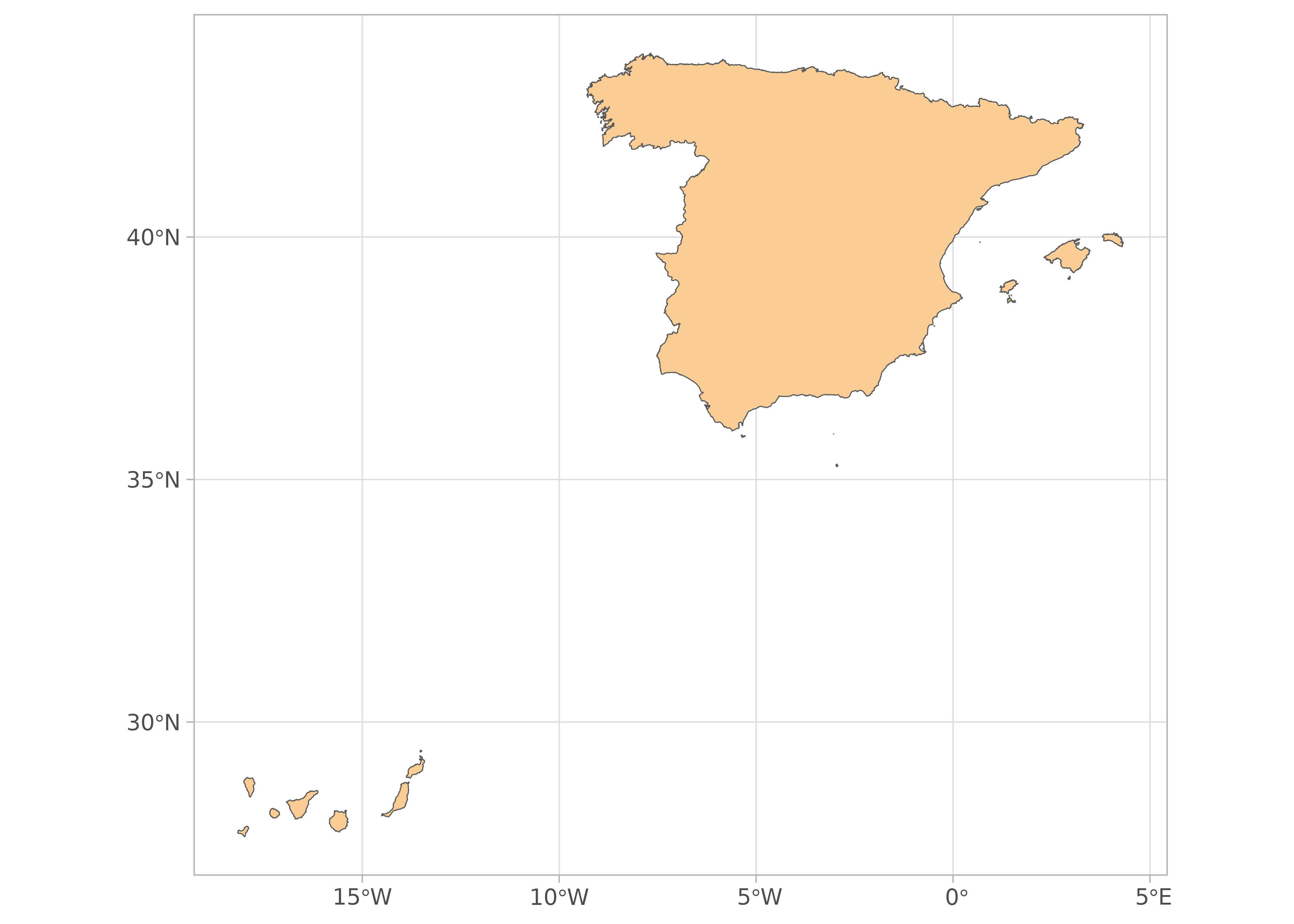
Displacing the Canary Islands
By default, most mapSpain functions move the Canary Islands closer to the mainland to improve visualization. Disable this behavior with moveCAN = FALSE when you need geometries in their original position.
The package also provides helpers for drawing boxes around the inset map. See the examples in the reference page.
esp_can <- esp_get_spain()
can_prov <- esp_get_can_provinces()
can_box <- esp_get_can_box()

ggplot(esp_can) +
  geom_sf() +
  geom_sf(data = can_prov) +
  geom_sf(data = can_box)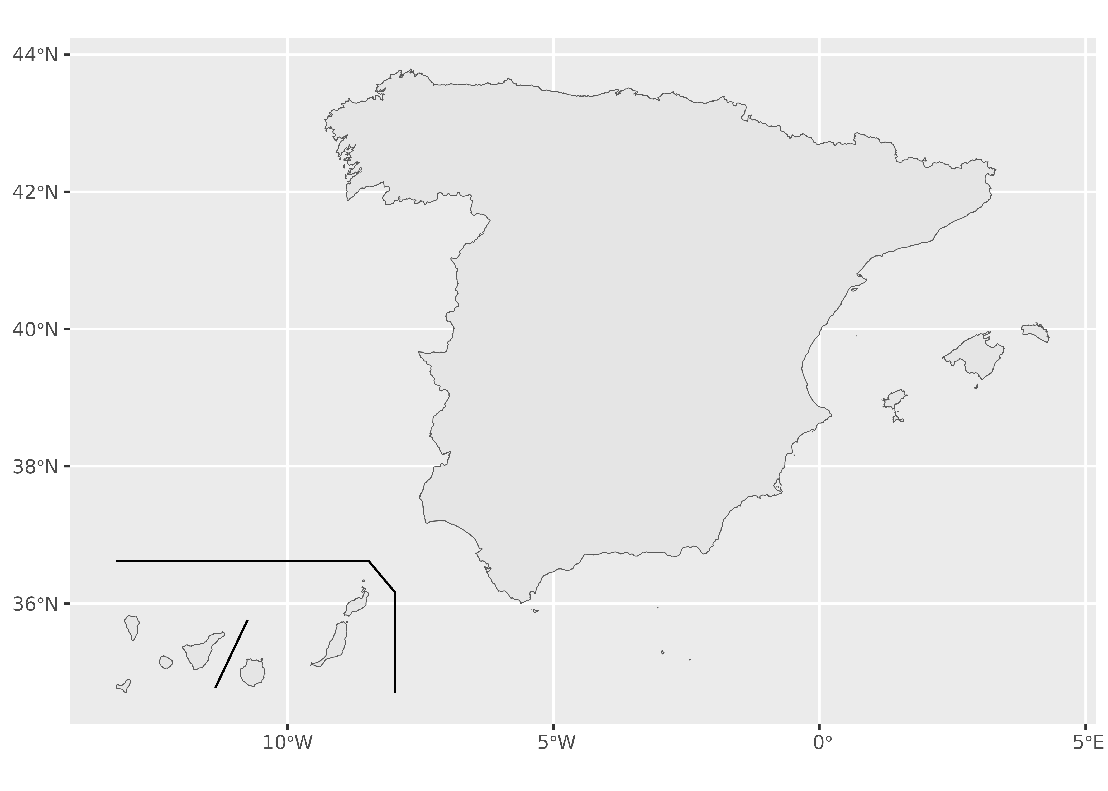
Use moveCAN = FALSE when working with static map tiles, interactive maps or spatial analysis.
NUTS
nuts1 <- esp_get_nuts(resolution = 60, epsg = 3035, nuts_level = 1)

ggplot(nuts1) +
  geom_sf() +
  labs(title = "NUTS 1: low resolution")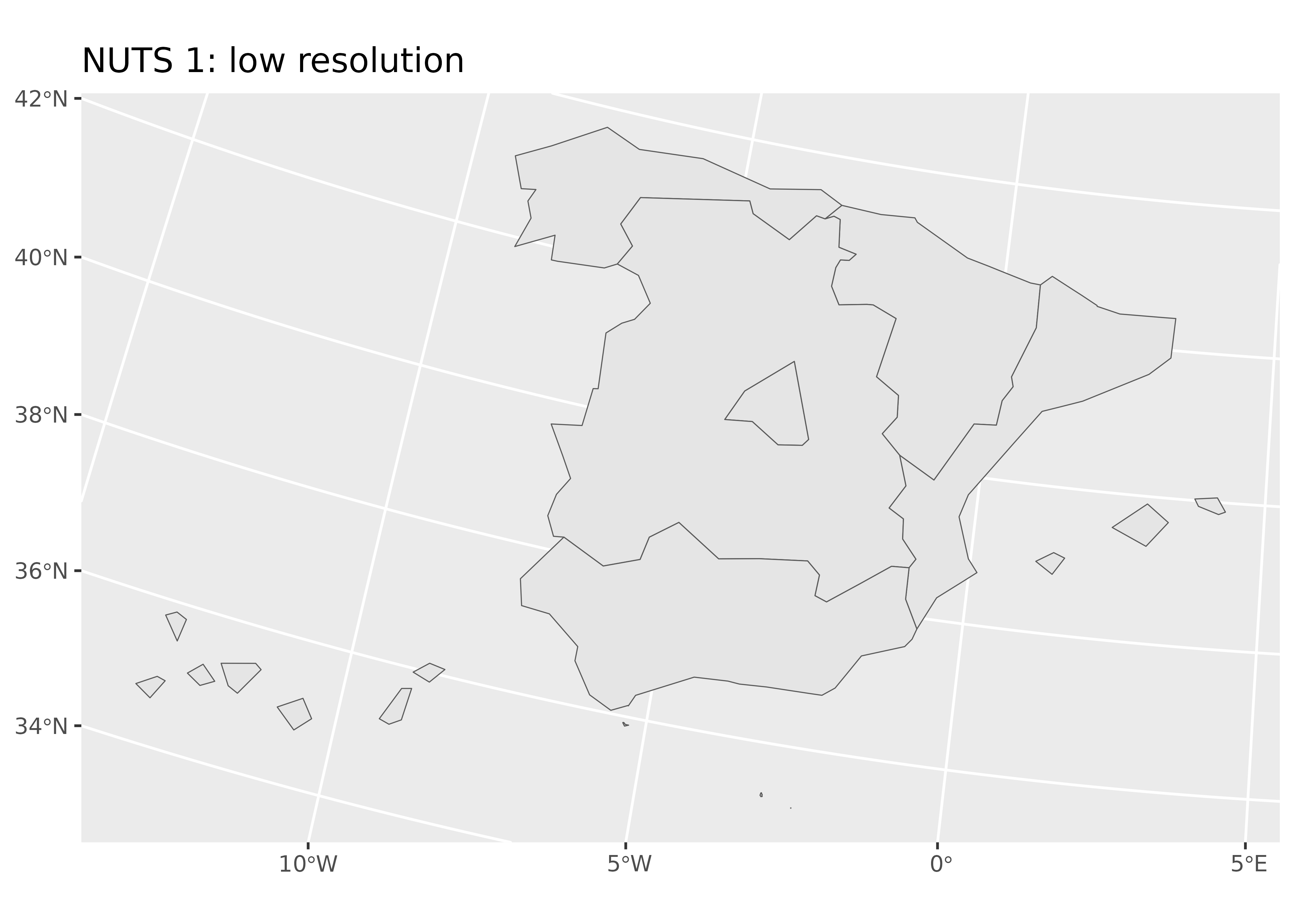
# Balearic Islands NUTS 3.
nuts3_baleares <- c("ES531", "ES532", "ES533")
paste(esp_dict_region_code(nuts3_baleares, "nuts"), collapse = ", ")
#> [1] "Eivissa y Formentera, Mallorca, Menorca"

nuts3_sf <- esp_get_nuts(region = nuts3_baleares, resolution = 1)

ggplot(nuts3_sf) +
  geom_sf(aes(fill = NAME_LATN)) +
  labs(fill = "Balearic Islands: NUTS 3") +
  scale_fill_viridis_d() +
  theme_minimal()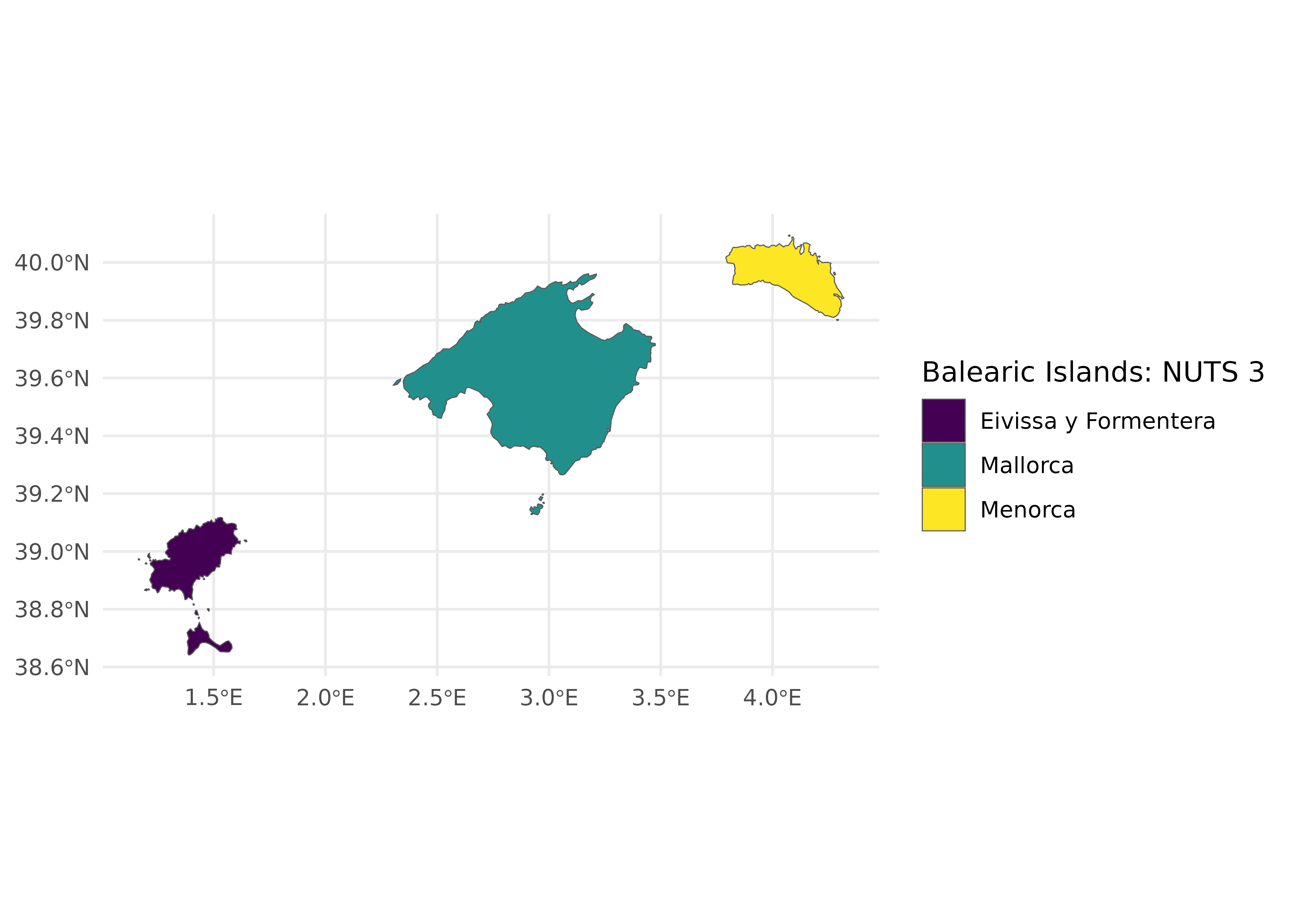
Autonomous Communities and Cities
ccaa <- esp_get_ccaa(
  ccaa = c(
    "Catalunya",
    "Comunidad Valenciana",
    "Aragón",
    "Baleares"
  ),
  resolution = 3
)

ccaa <- ccaa |>
  mutate(ccaa_cat = esp_dict_translate(ine.ccaa.name, "ca"))

ggplot(ccaa) +
  geom_sf(aes(fill = ccaa_cat)) +
  labs(fill = "Autonomous Communities and Cities") +
  theme_minimal() +
  scale_fill_discrete(type = hcl.colors(4, "Plasma"))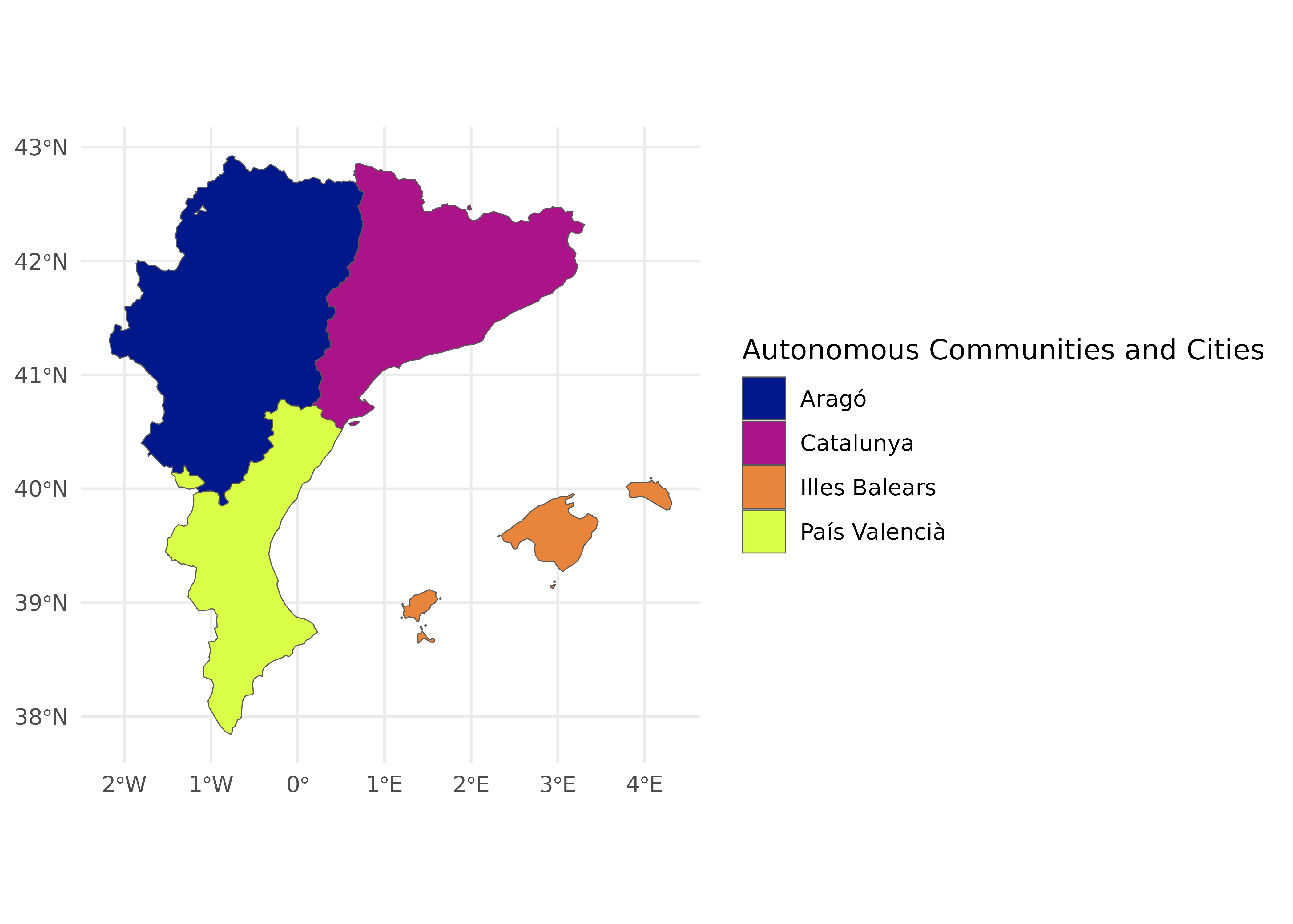
Provinces from SIANE
Passing a higher-level entity, such as Andalusia, returns all provinces within that entity.
provs <- esp_get_prov_siane(c(
  "Andalucía",
  "Ciudad Real",
  "Murcia",
  "Ceuta",
  "Melilla"
))

ggplot(provs) +
  geom_sf(aes(fill = prov.shortname.es), alpha = 0.9) +
  scale_fill_discrete(type = hcl.colors(12, "Cividis")) +
  theme_minimal() +
  labs(fill = "Provinces")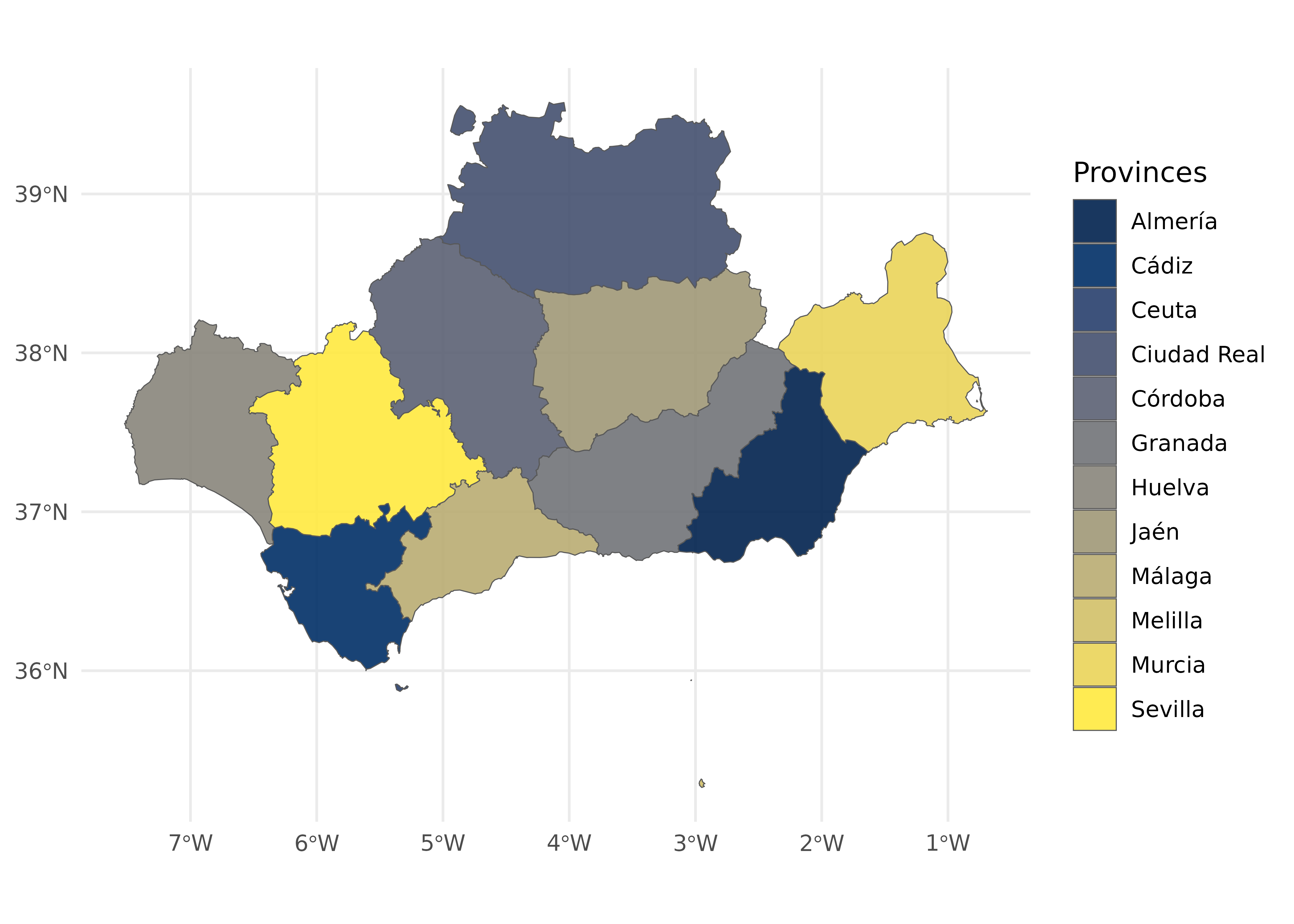
Municipalities
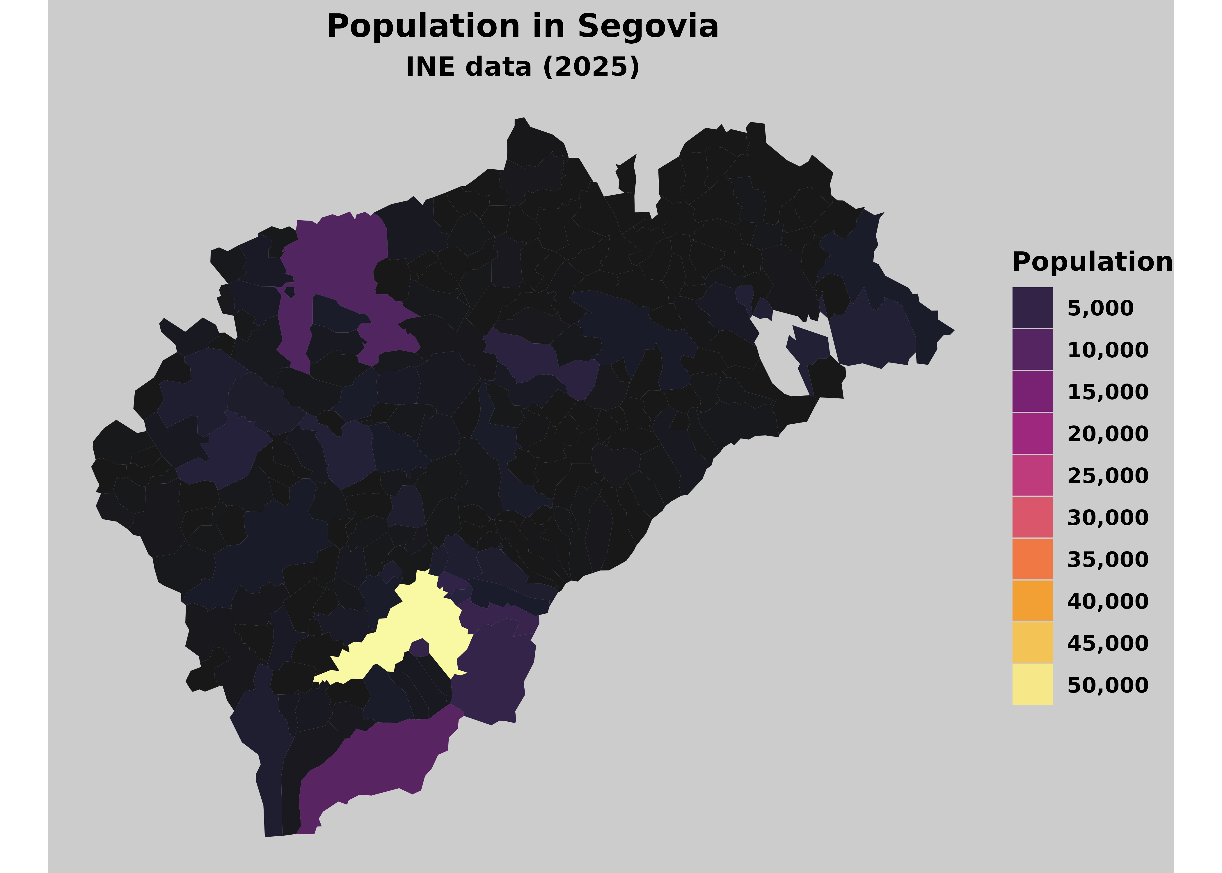
population <- mapSpain::pobmun25 |>
  select(-name)

munic <- esp_get_munic_siane(region = "Segovia", cache_dir = "./maps_spain/") |>
  # Example data: INE population.
  left_join(
    population,
    by = c("cpro", "cmun")
  )

ggplot(munic) +
  geom_sf(aes(fill = pob25), alpha = 0.9, color = NA) +
  scale_fill_gradientn(
    colors = hcl.colors(100, "Inferno"),
    n.breaks = 10,
    labels = scales::label_comma(),
    guide = guide_legend()
  ) +
  labs(
    fill = "Population",
    title = "Population in Segovia",
    subtitle = "INE data (2025)"
  ) +
  theme_void() +
  theme(
    plot.background = element_rect("grey80"),
    text = element_text(face = "bold"),
    plot.title = element_text(hjust = 0.5),
    plot.subtitle = element_text(hjust = 0.5)
  )
Grid maps
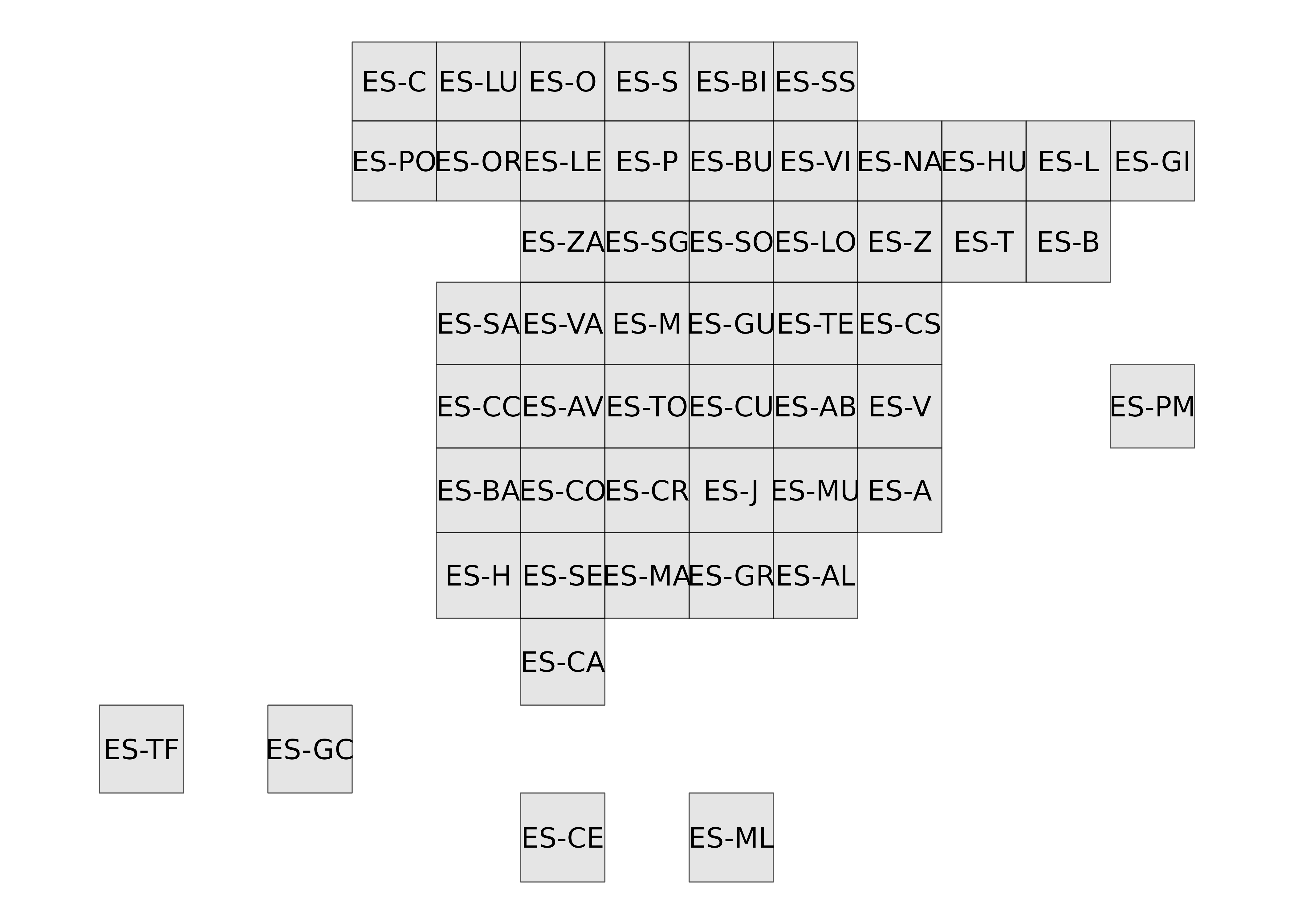
Grid maps are available as squares and hexagons for provinces and Autonomous Communities and Cities.
cuad <- esp_get_hex_ccaa()
hex <- esp_get_grid_prov()

ggplot(cuad) +
  geom_sf() +
  geom_sf_text(aes(label = iso2.ccaa.code)) +
  theme_void()

ggplot(hex) +
  geom_sf() +
  geom_sf_text(aes(label = iso2.prov.code)) +
  theme_void()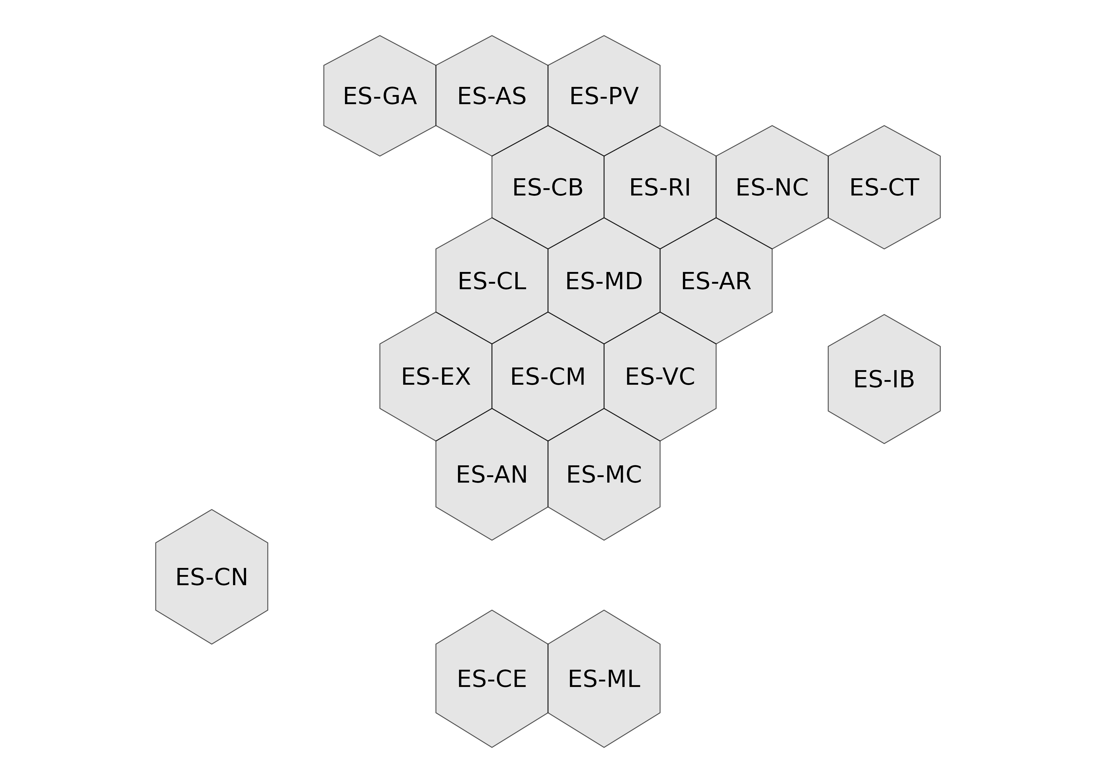
Static map tiles and imagery
mapSpain can also use static map tiles, such as satellite imagery, basemaps and roads, provided by different public institutions (https://www.idee.es/web/idee/segun-tipo-de-servicio).
These tiles can be used to create static maps as three- or four-band raster layers or as backgrounds for interactive maps through the leaflet package.
The providers come from the leaflet-providersESP plugin for leaflet.
Creating maps with static map tiles
Several options are available for composing maps with static map tiles:
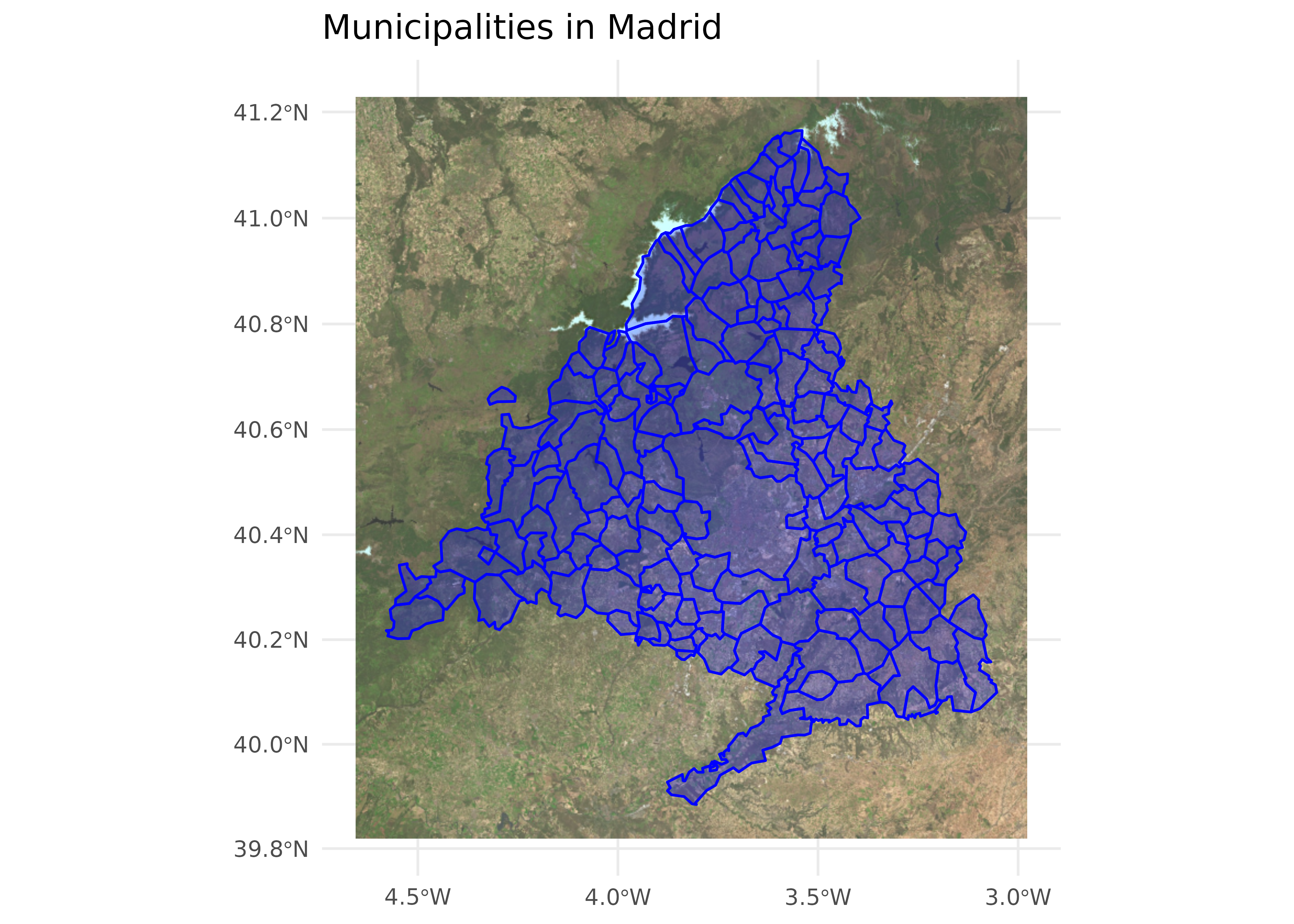
madrid_munis <- esp_get_munic_siane(region = "Madrid", epsg = 3857)
base_pnoa <- esp_get_tiles(madrid_munis, "PNOA",
  bbox_expand = 0.1,
  zoommin = 1, cache_dir = "./maps_spain/"
)

library(tidyterra)

ggplot() +
  geom_spatraster_rgb(data = base_pnoa) +
  geom_sf(
    data = madrid_munis,
    color = "blue",
    fill = "blue",
    alpha = 0.25,
    linewidth = 0.5
  ) +
  theme_minimal() +
  labs(title = "Municipalities in Madrid")

# Use the `mask` option.
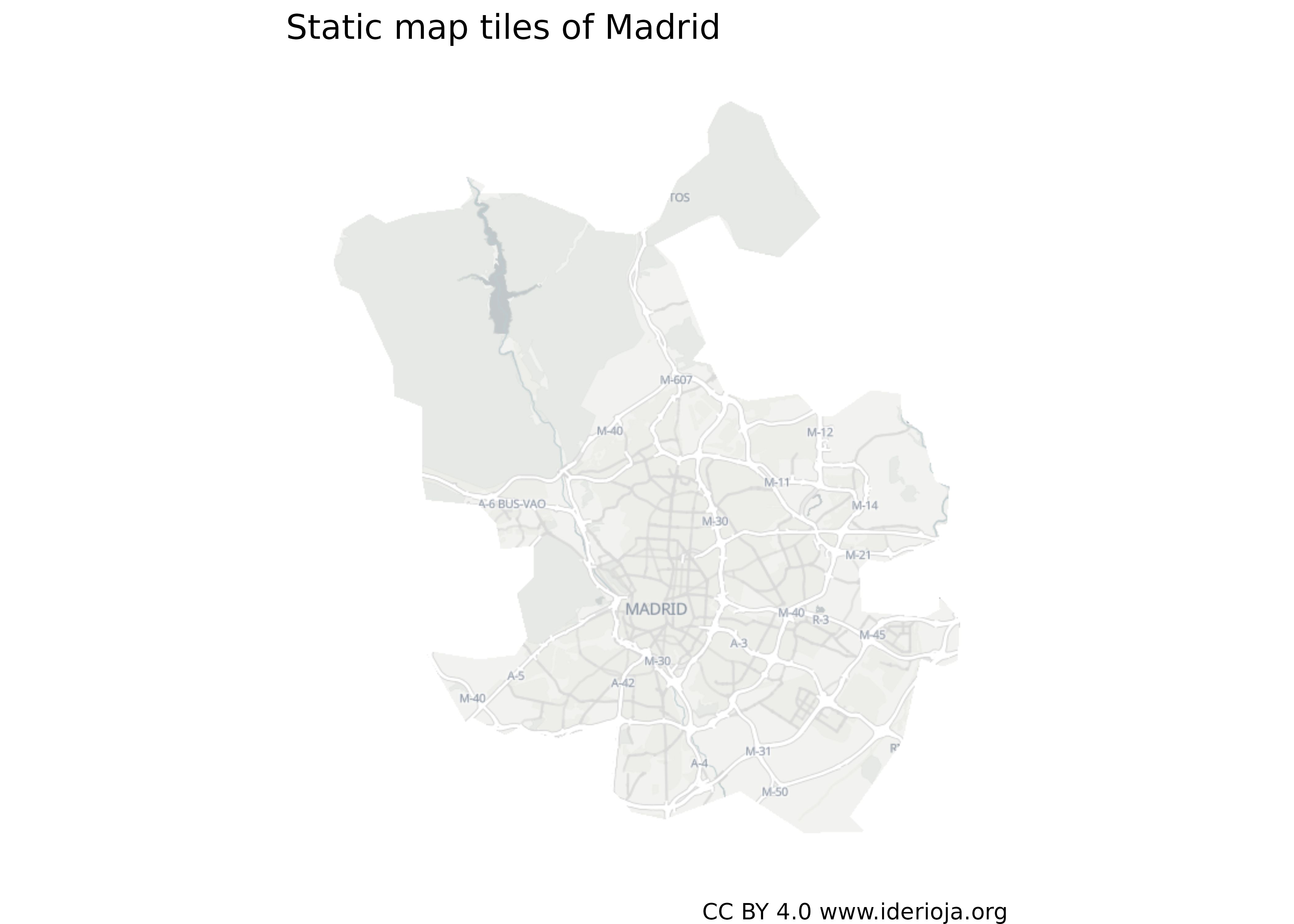
madrid <- esp_get_munic_siane(munic = "^Madrid$", epsg = 3857)

madrid_mask <- esp_get_tiles(
  madrid,
  "IDErioja.Claro",
  mask = TRUE,
  crop = TRUE,
  zoommin = 2,
  cache_dir = "./maps_spain/"
)

ggplot() +
  geom_spatraster_rgb(data = madrid_mask) +
  theme_void() +
  labs(
    title = "Static map tiles of Madrid",
    caption = "CC BY 4.0 www.iderioja.org"
  )
Dynamic maps with leaflet
Static map tiles can be used as backgrounds in static and interactive maps.
stations <- esp_get_railway(spatialtype = "point", epsg = 4326)

library(leaflet)
# Create an icon.

iconurl <- "https://ropenspain.github.io/mapSpain/icons/train.png"

train_icon <- makeIcon(iconurl, iconurl, 18, 18)
station_popups <- sprintf(
  "<strong>%s</strong>",
  stations$rotulo
) |>
  lapply(htmltools::HTML)

leaflet(stations, elementId = "railway", width = "100%", height = "60vh") |>
  addProviderEspTiles("IDErioja.Claro", group = "Base") |>
  addProviderEspTiles("MTN", group = "MTN") |>
  addProviderEspTiles("RedTransporte.Carreteras", group = "Roads") |>
  addProviderEspTiles(
    "RedTransporte.Ferroviario",
    group = "Railway lines"
  ) |>
  addMarkers(
    icon = train_icon,
    group = "Stations",
    popup = station_popups
  ) |>
  addLayersControl(
    baseGroups = c("Base", "MTN"),
    overlayGroups = c("Stations", "Railway lines", "Roads"),
    options = layersControlOptions(collapsed = FALSE)
  ) |>
  hideGroup(c("Railway lines", "Roads"))
Other resources
mapSpain includes additional functions for retrieving terrain, inland waters and river basin districts, as well as Spanish transport infrastructure such as roads, railway lines and stations.