Introduction
Tip
For more examples and vignettes, see the full site at https://ropenspain.github.io/mapSpain/.
mapSpain provides administrative boundaries and static map tiles for Spain.
mapSpain provides sf objects for Autonomous Communities and Cities, provinces, municipalities and NUTS levels in Spain. It also provides grid maps and complementary geometries, such as inset boxes and outlines for the Canary Islands.
mapSpain provides access to static map tiles from Spanish public administrations. Tiles can be represented on static maps with mapSpain::esp_get_tiles() or on an interactive leaflet map with mapSpain::addProviderEspTiles().
mapSpain also includes a dictionary that translates Spanish subdivision names to English, Spanish, Catalan, Basque and Galician. It also converts names among coding standards such as NUTS, ISO2 and INE codes.
Caching
mapSpain provides data and tile caching. Set a cache directory with:
esp_set_cache_dir("./path/to/location")mapSpain relies on giscoR for downloading some files, and both packages can share cache settings. Using the same cache directory for both packages speeds up data loading in your session.
Basic example
These examples show key mapSpain workflows:
library(mapSpain)
library(ggplot2)

country <- esp_get_spain()
lines <- esp_get_can_box()

ggplot(country) +
  geom_sf(fill = "cornsilk", color = "#887e6a") +
  labs(title = "Map of Spain") +
  theme(
    panel.background = element_rect(fill = "#fffff3"),
    panel.border = element_rect(
      colour = "#887e6a",
      fill = NA,
    ),
    text = element_text(
      family = "serif",
      face = "bold"
    )
  )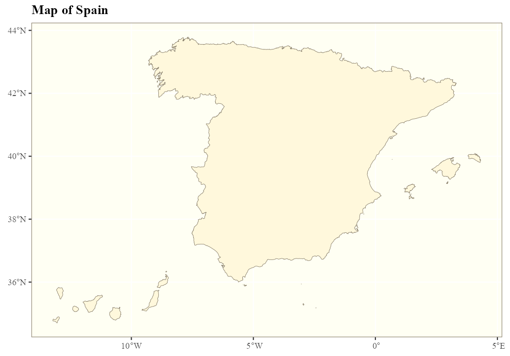
Example: map of Spain
# Plot provinces.

andalucia <- esp_get_prov_siane("Andalucia")

ggplot(andalucia) +
  geom_sf(fill = "darkgreen", color = "white") +
  theme_bw()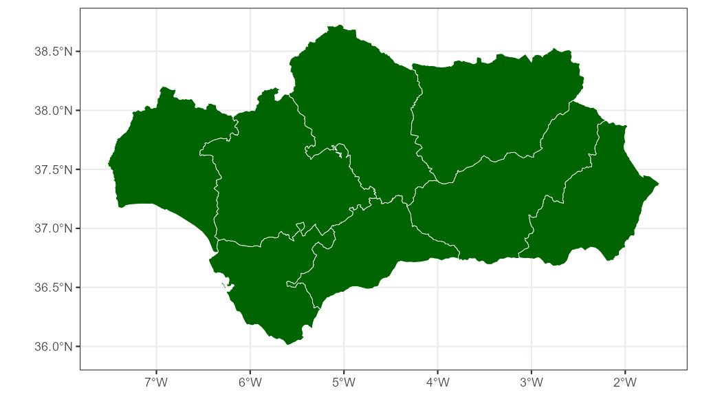
Example: provinces of Andalusia
# Plot municipalities.

euskadi_ccaa <- esp_get_ccaa_siane("Euskadi")
euskadi <- esp_get_munic_siane(region = "Euskadi")

# Use the dictionary.

euskadi$name_eu <- esp_dict_translate(euskadi$ine.prov.name, lang = "eu")

ggplot(euskadi_ccaa) +
  geom_sf(fill = "grey50") +
  geom_sf(data = euskadi, aes(fill = name_eu)) +
  scale_fill_manual(values = c("red2", "darkgreen", "ivory2")) +
  labs(
    fill = "",
    title = "Euskal Autonomia Erkidegoko",
    subtitle = "Probintziak"
  ) +
  theme_void() +
  theme(
    plot.title = element_text(face = "bold"),
    plot.subtitle = element_text(face = "italic")
  )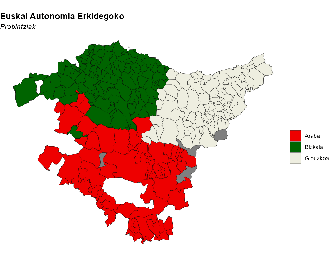
Example: municipalities of the Basque Country
Choropleth and label maps
Analyze the distribution of women in each Autonomous Community or City with ggplot2:
library(dplyr)

census <- mapSpain::pobmun25 |>
  select(-name)

# Extract Autonomous Community or City codes from the base dataset.
codelist <- mapSpain::esp_codelist |>
  select(cpro, codauto) |>
  distinct()

census_ccaa <- census |>
  left_join(codelist) |>
  # Summarize by Autonomous Community or City.
  group_by(codauto) |>
  summarise(pob25 = sum(pob25), men = sum(men), women = sum(women)) |>
  mutate(
    porc_women = women / pob25,
    porc_women_lab = paste0(round(100 * porc_women, 2), "%")
  )

# Merge into spatial data.
ccaa_sf <- esp_get_ccaa() |>
  left_join(census_ccaa)

can <- esp_get_can_box()

# Plot with ggplot.
library(ggplot2)

ggplot(ccaa_sf) +
  geom_sf(aes(fill = porc_women), color = "grey70", linewidth = 0.3) +
  geom_sf(data = can, color = "grey70") +
  geom_sf_label(
    aes(label = porc_women_lab),
    fill = "white",
    alpha = 0.5,
    size = 3,
    linewidth = 0
  ) +
  scale_fill_gradientn(
    colors = hcl.colors(10, "Blues", rev = TRUE),
    n.breaks = 10,
    labels = scales::label_percent(),
    guide = guide_legend(title = "% women", position = "inside")
  ) +
  theme_void() +
  theme(legend.position.inside = c(0.1, 0.6)) +
  labs(caption = "Source: CartoBase ANE 2006-2024 CC-BY 4.0 ign.es, INE")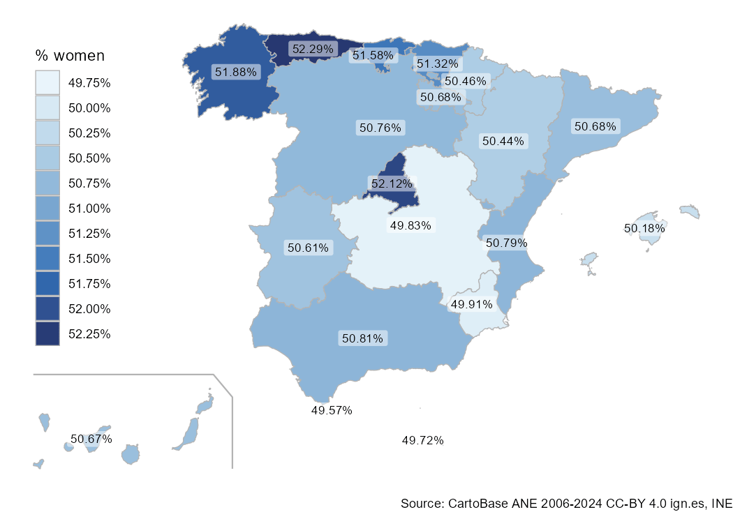
Percentage of women by Autonomous Communities and Cities (2025)
Thematic maps
This example shows how mapSpain can be used to create thematic maps. For plotting, we use the ggplot2 package, though any package that works with sf objects, such as tmap, mapsf or leaflet, could also be used.
# Calculate population density in Spain.
library(sf)

pop <- mapSpain::pobmun25 |>
  select(-name)

munic <- esp_get_munic_siane(rawcols = TRUE) |>
  # Use the area field available in the SIANE data.
  mutate(area_km2 = st_area_sh * 10000)

munic_pop <- munic |>
  left_join(pop) |>
  mutate(dens = pob25 / area_km2)

br <- c(-Inf, 10, 25, 100, 200, 500, 1000, 5000, 10000, Inf)

munic_pop$cuts <- cut(munic_pop$dens, br)

ggplot(munic_pop) +
  geom_sf(aes(fill = cuts), color = NA, linewidth = 0) +
  scale_fill_manual(
    values = c("grey5", hcl.colors(length(br) - 2, "Spectral")),
    labels = prettyNum(c(0, br[-1]), big.mark = ","),
    guide = guide_legend(
      title = "People per km2",
      direction = "horizontal",
      nrow = 1
    )
  ) +
  labs(title = "Population density in Spain (2025)") +
  theme_void() +
  theme(
    plot.title = element_text(hjust = 0.5),
    plot.background = element_rect(fill = "black"),
    text = element_text(colour = "white"),
    legend.position = "bottom",
    legend.title.position = "top",
    legend.text.position = "bottom",
    legend.key.width = unit(30, "pt")
  ) +
  labs(caption = "Source: CartoBase ANE 2006-2024 CC-BY 4.0 ign.es, INE")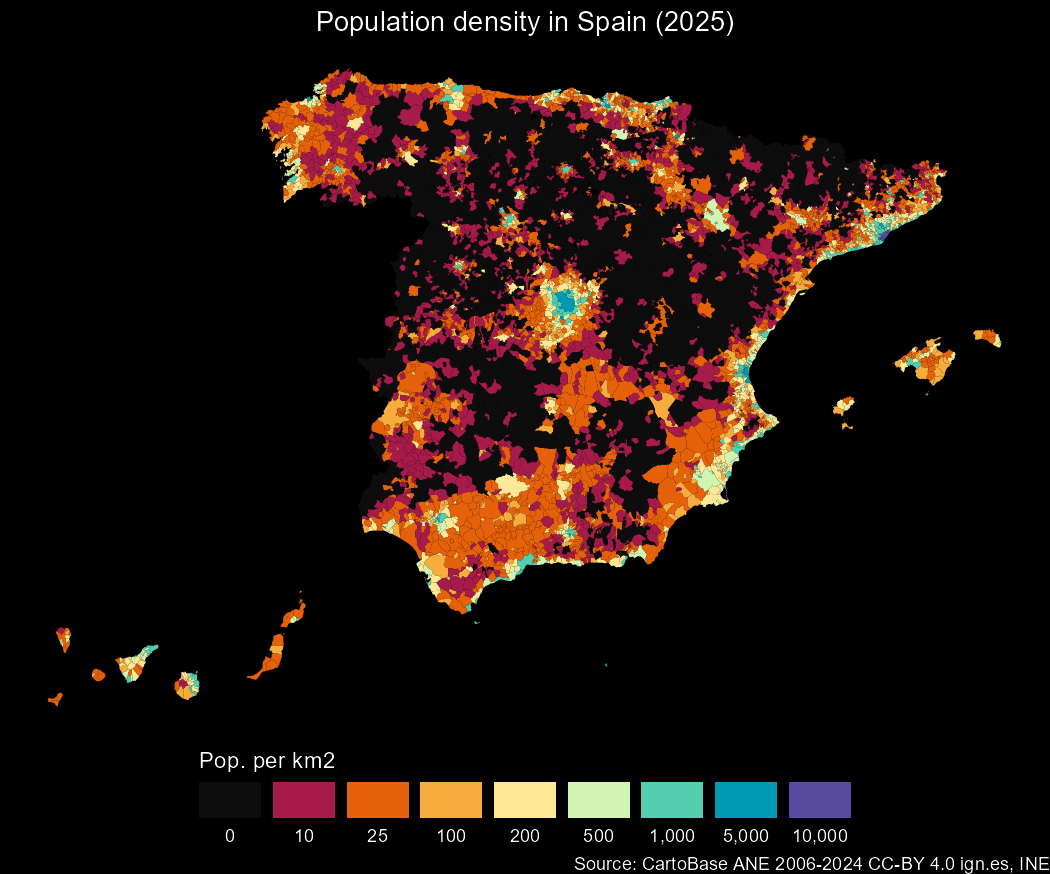
Population density in Spain (2025)
mapSpain and giscoR
If you need to plot Spain alongside other countries, use the giscoR package, which is installed as a dependency of mapSpain. Here is a basic example:
library(giscoR)

# Use the same resolution for aligned boundaries.
res <- 3

all_countries <- gisco_get_countries(resolution = res) |>
  st_transform(3035)

eu_countries <- gisco_get_countries(
  resolution = res,
  region = "EU"
) |>
  st_transform(3035)

ccaa <- esp_get_ccaa(
  moveCAN = FALSE,
  resolution = res
) |>
  st_transform(3035)

# Plot.
ggplot(all_countries) +
  geom_sf(fill = "#DFDFDF", color = "#656565") +
  geom_sf(data = eu_countries, fill = "#FDFBEA", color = "#656565") +
  geom_sf(data = ccaa, fill = "#C12838", color = "grey80", linewidth = 0.1) +
  # Center on Europe: EPSG 3035.
  coord_sf(
    xlim = c(2377294, 7453440),
    ylim = c(1313597, 5628510)
  ) +
  theme(
    panel.background = element_blank(),
    panel.grid = element_line(
      colour = "#DFDFDF",
      linetype = "dotted"
    )
  ) +
  labs(caption = giscoR::gisco_attributions("es"))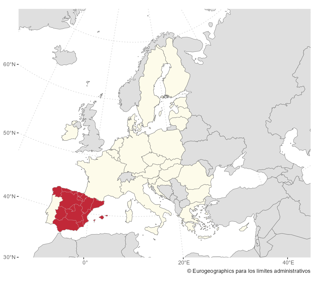
mapSpain and giscoR example
Working with static map tiles
mapSpain provides an interface for working with static map tiles. It can download tiles as .png or .jpeg, depending on the tile service, and use them alongside your sf objects.
mapSpain also includes a plugin for leaflet maps, which lets you add Spanish public administration basemaps to interactive maps.
The services are implemented with the leaflet-providersESP Leaflet plugin. Its provider catalog lists all available services.
Note
When working with static map tiles, set
moveCAN = FALSEinesp_get_*()functions. Seeesp_move_can()for details.