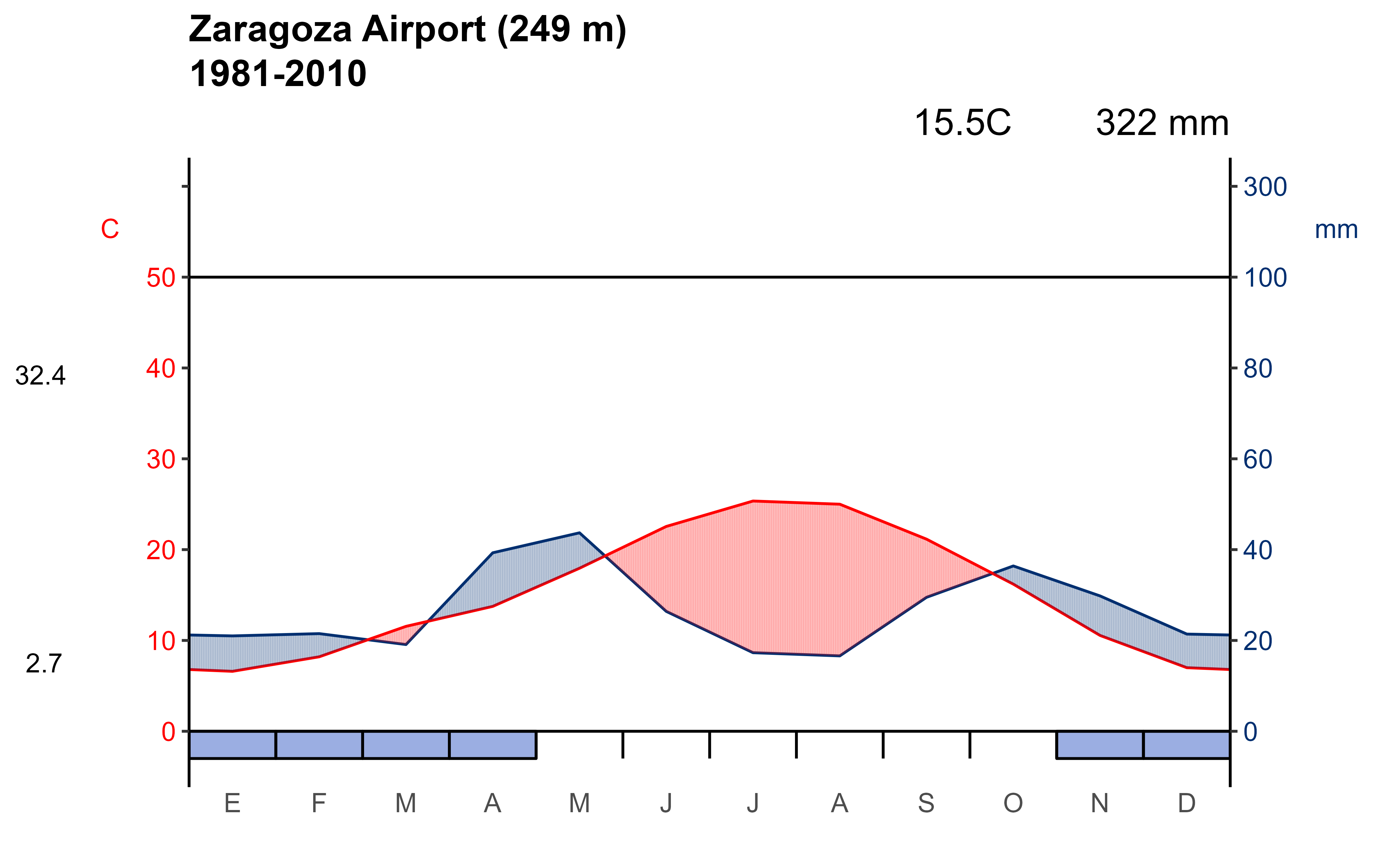
Plots a Walter-Lieth climate diagram for a station using ggplot2.
Usage
ggclimat_walter_lieth(
  dat,
  est = "",
  alt = NA,
  per = NA,
  mlab = "es",
  pcol = "#002F70",
  tcol = "#ff0000",
  pfcol = "#9BAEE2",
  sfcol = "#3C6FC4",
  shem = FALSE,
  p3line = FALSE,
  ...
)
Arguments
- dat
A data frame containing monthly climatology data.
- est
A character string with the climatological station name.
- alt
A numeric value with the station altitude in meters.
- per
A character string describing the averaging period.
- mlab
Month labels for the x-axis. Use a two-letter language code, such as
"en"or"es". Seereadr::locale()for details.- pcol
A color for precipitation.
- tcol
A color for temperature.
- pfcol
A fill color for probable frosts.
- sfcol
A fill color for certain frosts.
- shem
A logical value. If
TRUE, plots a Southern Hemisphere station.- p3line
Set to
TRUEto draw a supplementary precipitation line relative to three times the temperature (as suggested by Bogdan Rosca).- ...
Further graphic arguments.
Value
A ggplot object.
Details
![[Experimental]](figures/lifecycle-experimental.svg)
See the details in climatol::diagwl().
Climatology data must be passed as a 4 by 12 matrix or data frame of monthly data from January to December. Rows must contain mean precipitation, mean maximum daily temperature, mean minimum daily temperature and absolute monthly minimum temperature, in that order.
See climaemet_9434_climatogram for a sample dataset.
References
Walter H, Lieth H (1967). Klimadiagramm-Weltatlas. VEB Gustav Fischer Verlag, Jena. Published in three installments, 1960-1967, https://hdl.handle.net/2268.1/7079.
Guijarro JA (2026). climatol: Climate Tools (Series Homogenization and Derived Products). doi:10.32614/CRAN.package.climatol . R package version 4.5-0, https://CRAN.R-project.org/package=climatol.
See also
climatol::diagwl()provides the original diagram implementation.readr::locale()provides language-specific month labels.
Walter-Lieth climate diagrams:
climatogram_normal(),
climatogram_period()
Examples
library(ggplot2)
wl <- ggclimat_walter_lieth(
climaemet::climaemet_9434_climatogram,
alt = "249",
per = "1981-2010",
est = "Zaragoza Airport"
)
wl
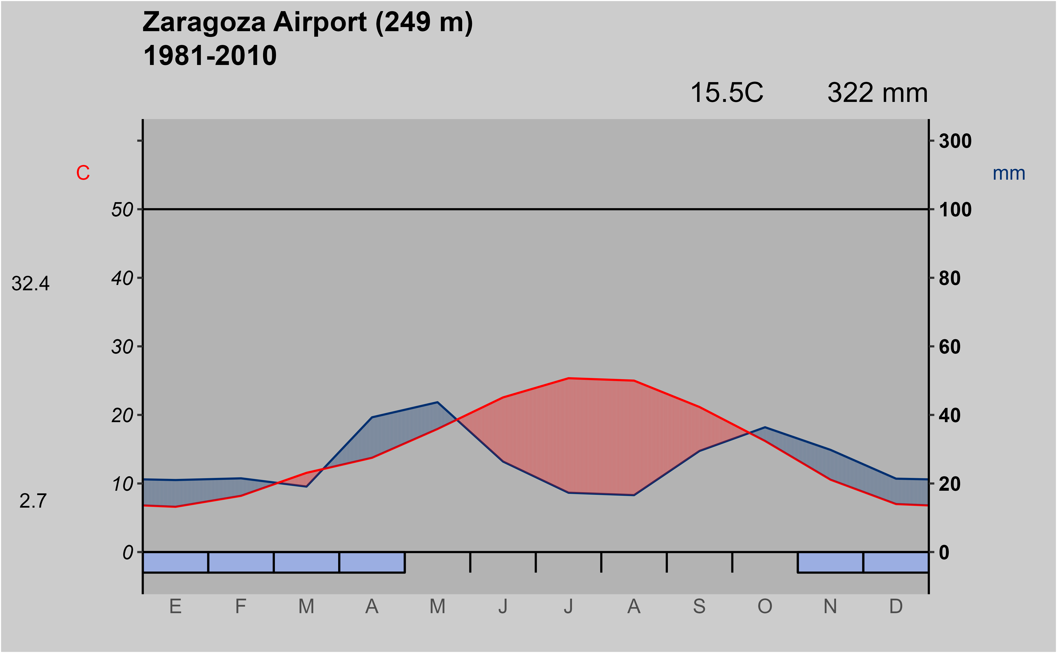
 # Modify the ggplot object.
wl + theme(
plot.background = element_rect(fill = "grey80"),
panel.background = element_rect(fill = "grey70"),
axis.text.y.left = element_text(
colour = "black",
face = "italic"
),
axis.text.y.right = element_text(
colour = "black",
face = "bold"
)
)
# Modify the ggplot object.
wl + theme(
plot.background = element_rect(fill = "grey80"),
panel.background = element_rect(fill = "grey70"),
axis.text.y.left = element_text(
colour = "black",
face = "italic"
),
axis.text.y.right = element_text(
colour = "black",
face = "bold"
)
)