Get started with tidyBdE

tidyBdE is an R package that retrieves time series data from Banco de España bulk CSV files and the Statistics web service (API). Data are returned as tibble objects. The package infers date, character and numeric column types where possible. Bulk CSV functions use stable sequential numbers (Numero_secuencial), while API functions use API series codes (Nombre_de_la_serie).

Search for time series

Banco de España (BdE) publishes numerous time series produced by the institution or compiled from other sources, such as Eurostat or INE.

Catalog metadata is the main entry point for discovering time series. You can search for time series by name:

library(tidyBdE)

library(ggplot2)
library(dplyr)
library(tidyr)

# Search for GBP in the "TC" (exchange rate) catalog metadata.
xr_gbp <- bde_catalog_search("GBP", catalog = "TC")

xr_gbp |>
  select(Numero_secuencial, Descripcion_de_la_serie) |>
  # Display the table in the document.
  knitr::kable()

Numero_secuencial	Descripcion_de_la_serie
573214	Tipos de cambio. Libras esterlinas por euro (GBP/EUR)

Table 1: Search results

Note: BdE catalog metadata is currently available in Spanish only, so search terms must be in Spanish to retrieve results.

After you find a time series, load the EUR/GBP exchange rate from bulk CSV files using its stable sequential number (Numero_secuencial):

seq_number <- xr_gbp |>
  # Select the first record.
  slice(1) |>
  # Get the stable sequential number.
  pull(Numero_secuencial) |>
  # Convert to numeric.
  as.double()

seq_number
#> [1] 573214

time_series <- bde_series_load(seq_number, series_label = "EUR_GBP_XR") |>
  filter(Date >= "2010-01-01" & Date <= "2020-12-31") |>
  drop_na()

time_series
#> # A tibble: 2,816 × 2
#>    Date       EUR_GBP_XR
#>    <date>          <dbl>
#>  1 2010-01-04      0.891
#>  2 2010-01-05      0.900
#>  3 2010-01-06      0.899
#>  4 2010-01-07      0.900
#>  5 2010-01-08      0.893
#>  6 2010-01-11      0.899
#>  7 2010-01-12      0.897
#>  8 2010-01-13      0.895
#>  9 2010-01-14      0.890
#> 10 2010-01-15      0.881
#> # ℹ 2,806 more rows

Plot time series

tidyBdE provides a custom ggplot2 theme based on BdE publications:

ggplot(time_series, aes(x = Date, y = EUR_GBP_XR)) +
  geom_line(colour = bde_tidy_palettes(n = 1)) +
  geom_smooth(method = "gam", colour = bde_tidy_palettes(n = 2)[2]) +
  labs(
    title = "EUR/GBP exchange rate (2010-2020)",
    subtitle = "%",
    caption = "Source: BdE"
  ) +
  geom_vline(
    xintercept = as.Date("2016-06-23"),
    linetype = "dotted"
  ) +
  geom_label(aes(
    x = as.Date("2016-06-23"),
    y = 0.95,
    label = "Brexit"
  )) +
  coord_cartesian(ylim = c(0.7, 1)) +
  theme_tidybde()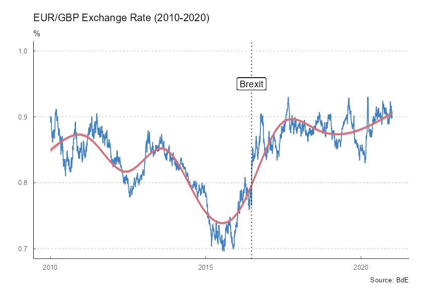

Figure 1: EUR/GBP exchange rate (2010-2020)

Convenience functions retrieve selected Spanish macroeconomic indicators, so you do not need to search for them manually:

# Data in long format.

plotseries <- bde_ind_gdp_var("GDP YoY", out_format = "long") |>
  bind_rows(
    bde_ind_unemployment_rate("Unemployment Rate", out_format = "long")
  ) |>
  drop_na() |>
  filter(Date >= "2010-01-01" & Date <= "2019-12-31")

ggplot(plotseries, aes(x = Date, y = serie_value)) +
  geom_line(aes(color = serie_name), linewidth = 1) +
  labs(
    title = "Spanish economic indicators (2010-2019)",
    subtitle = "%",
    caption = "Source: BdE"
  ) +
  theme_tidybde() +
  scale_color_bde_d(palette = "bde_vivid_pal") # Use a tidyBdE palette.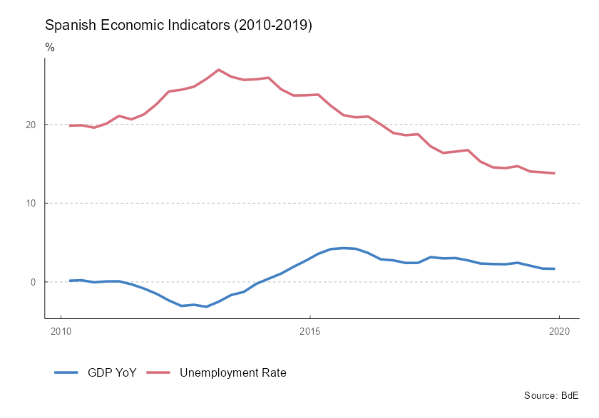

Figure 2: Spanish economic indicators (2010-2019)

Caching

Set the bde_cache_dir option to create a local cache:

options(bde_cache_dir = "./path/to/location")

When this option is set, tidyBdE uses bulk CSV files cached in the bde_cache_dir directory to speed up data retrieval.

Update cached data after monthly or quarterly releases with the following commands:

bde_catalog_update()

# Or use `update_cache = TRUE` in most functions.

bde_series_load(573214, update_cache = TRUE)