Load a single BdE time series.
The series alias is a positional code showing the location (column and/or row) of the series in the table. Although it is unique, it is not stable enough to identify a time series because it may change when the series moves.
To ensure series can still be identified after these changes, they are
assigned a sequential number, referred to as series_code in this function.
A single time series may appear in different tables, so it can have several
aliases. If you need to search by alias, use bde_series_full_load().
Usage
bde_series_load(
  series_code,
  series_label = NULL,
  out_format = "wide",
  parse_dates = TRUE,
  parse_numeric = TRUE,
  cache_dir = NULL,
  update_cache = FALSE,
  verbose = FALSE,
  extract_metadata = FALSE
)
Arguments
- series_code
Numeric value, value coercible with
base::as.double(), or vector of time series codes from theNúmero secuencialfield of the corresponding series. Seebde_catalog_load().- series_label
Optional character string or vector of labels to assign to the extracted series.
- out_format
The format to return, either
"wide"or"long". See Value for details and the Examples section.- parse_dates
Logical. If
TRUE, date columns are parsed withbde_parse_dates().- parse_numeric
Logical. If
TRUE, the columns are parsed to double (numeric) values. See Note.- cache_dir
Path to a cache directory. The directory can also be set with
options(bde_cache_dir = "path/to/dir").- update_cache
Logical. If
TRUE, the requested file is refreshed incache_dir.- verbose
Logical. If
TRUE, display information useful for debugging.- extract_metadata
Logical. If
TRUE, the output is the metadata of the requested series.
Value
A tibble with a Date column:
With
out_format = "wide", each series is presented in a separate column with the name defined byseries_label.With
out_format = "long", the tibble has two additional columns:serie_name, with the label of each series, andserie_value, with the corresponding value.
"wide" format is more suitable for exporting to a .csv file, while
"long" format is more suitable for creating plots using
ggplot2::ggplot(). See also tidyr::pivot_longer() and
tidyr::pivot_wider().
Note
This function attempts to coerce the columns to numbers. For some time series, a warning may be displayed if the parsing fails.
See also
bde_catalog_load(),
bde_catalog_search(), bde_indicators()
Other series:
bde_series_full_load()
Examples
# \donttest{
# Show metadata.
bde_series_load(573234, verbose = TRUE, extract_metadata = TRUE)
#> ℹ Using temporary cache directory /tmp/RtmpZwkfOF.
#> ✔ Using cached catalog "BE".
#> ✔ Using cached catalog "SI".
#> ✔ Using cached catalog "TC".
#> ✔ Using cached catalog "TI".
#> ✔ Using cached catalog "PB".
#> ℹ Parsing date columns.
#> ℹ Extracting series 573234.
#> ℹ Downloading series 573234 from file TC_1_1.csv (alias "TC_1_1.1").
#> ℹ Using temporary cache directory /tmp/RtmpZwkfOF/TC.
#> ℹ Downloading file from <https://www.bde.es/webbe/es/estadisticas/compartido/datos/csv/tc_1_1.csv>.
#> # A tibble: 6 × 2
#> Date `573234`
#> <chr> <chr>
#> 1 CÓDIGO DE LA SERIE DTCCBCEUSDEUR.B
#> 2 NÚMERO SECUENCIAL 573234
#> 3 ALIAS DE LA SERIE TC_1_1.1
#> 4 DESCRIPCIÓN DE LA SERIE Tipo de cambio. Dólares estadounidenses por euro …
#> 5 DESCRIPCIÓN DE LAS UNIDADES Dólares de Estados Unidos por Euro
#> 6 FRECUENCIA LABORABLE
# Load data.
bde_series_load(573234, extract_metadata = FALSE)
#> # A tibble: 7,154 × 2
#> Date `573234`
#> <date> <dbl>
#> 1 1999-01-04 1.18
#> 2 1999-01-05 1.18
#> 3 1999-01-06 1.17
#> 4 1999-01-07 1.16
#> 5 1999-01-08 1.17
#> 6 1999-01-11 1.16
#> 7 1999-01-12 1.15
#> 8 1999-01-13 1.17
#> 9 1999-01-14 1.17
#> 10 1999-01-15 1.16
#> # ℹ 7,144 more rows
# Load multiple series.
bde_series_load(c(573234, 573214),
series_label = c("US/EUR", "GBP/EUR"),
extract_metadata = TRUE
)
#> # A tibble: 6 × 3
#> Date `US/EUR` `GBP/EUR`
#> <chr> <chr> <chr>
#> 1 CÓDIGO DE LA SERIE DTCCBCEUSDEUR.B DTCCBCEG…
#> 2 NÚMERO SECUENCIAL 573234 573214
#> 3 ALIAS DE LA SERIE TC_1_1.1 TC_1_1.4
#> 4 DESCRIPCIÓN DE LA SERIE Tipo de cambio. Dólares estadounidenses… Tipo de …
#> 5 DESCRIPCIÓN DE LAS UNIDADES Dólares de Estados Unidos por Euro Libras e…
#> 6 FRECUENCIA LABORABLE LABORABLE
wide <- bde_series_load(c(573234, 573214),
series_label = c("US/EUR", "GBP/EUR")
)
# Show wide output.
wide
#> # A tibble: 7,154 × 3
#> Date `US/EUR` `GBP/EUR`
#> <date> <dbl> <dbl>
#> 1 1999-01-04 1.18 0.711
#> 2 1999-01-05 1.18 0.712
#> 3 1999-01-06 1.17 0.708
#> 4 1999-01-07 1.16 0.706
#> 5 1999-01-08 1.17 0.709
#> 6 1999-01-11 1.16 0.704
#> 7 1999-01-12 1.15 0.707
#> 8 1999-01-13 1.17 0.708
#> 9 1999-01-14 1.17 0.706
#> 10 1999-01-15 1.16 0.704
#> # ℹ 7,144 more rows
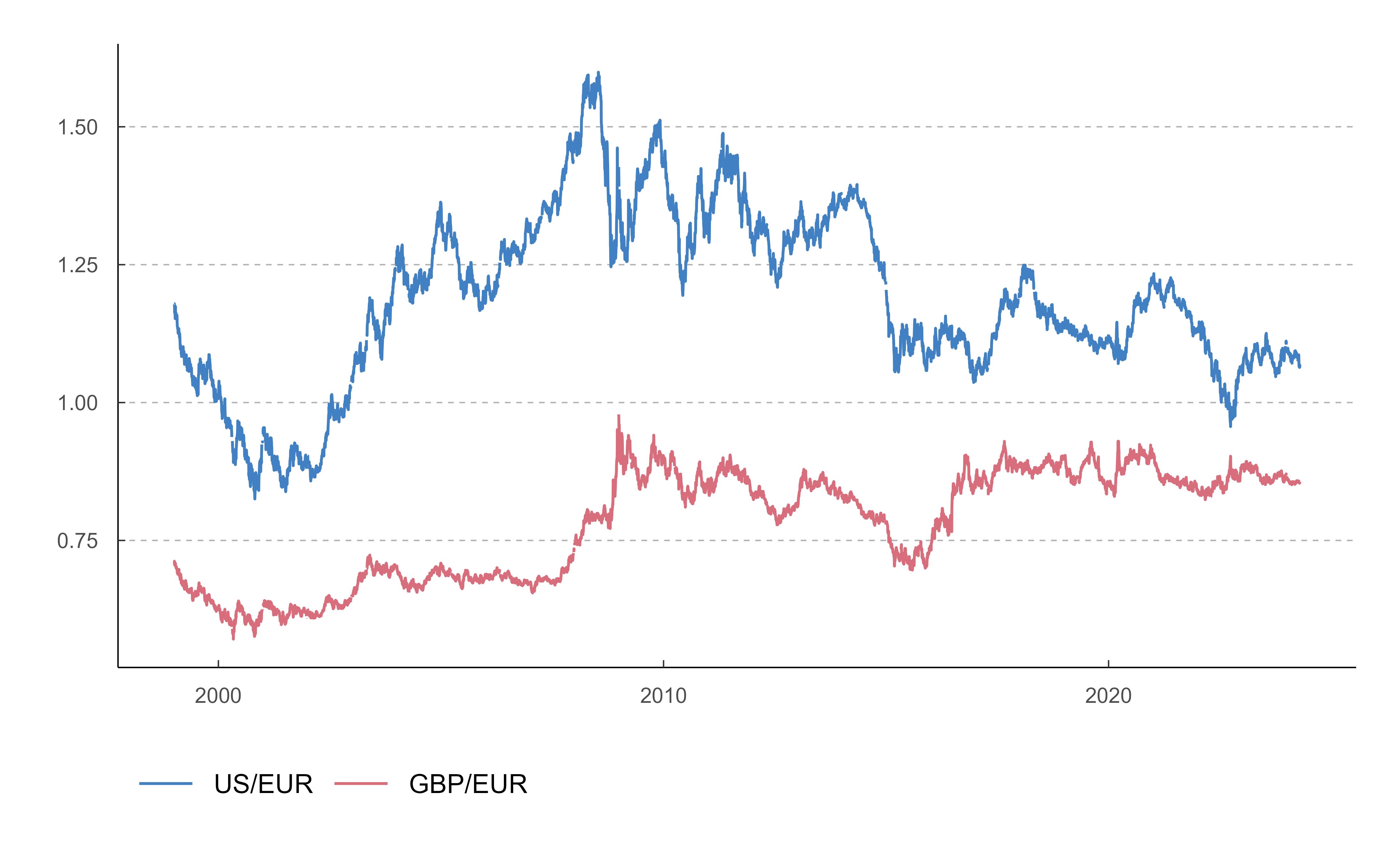
# Show long output.
long <- bde_series_load(c(573234, 573214),
series_label = c("US/EUR", "GBP/EUR"),
out_format = "long"
)
long
#> # A tibble: 14,308 × 3
#> Date serie_name serie_value
#> <date> <fct> <dbl>
#> 1 1999-01-04 US/EUR 1.18
#> 2 1999-01-05 US/EUR 1.18
#> 3 1999-01-06 US/EUR 1.17
#> 4 1999-01-07 US/EUR 1.16
#> 5 1999-01-08 US/EUR 1.17
#> 6 1999-01-11 US/EUR 1.16
#> 7 1999-01-12 US/EUR 1.15
#> 8 1999-01-13 US/EUR 1.17
#> 9 1999-01-14 US/EUR 1.17
#> 10 1999-01-15 US/EUR 1.16
#> # ℹ 14,298 more rows
# Use with `ggplot2`.
library(ggplot2)
ggplot(long, aes(Date, serie_value)) +
geom_line(aes(group = serie_name, color = serie_name)) +
scale_color_bde_d() +
theme_tidybde()
 # }
# }