BdE scales for ggplot2.

Scales to be used with the ggplot2 package. Discrete palettes are named as scale_*_bde_d while continuous palettes are named scale_*_bde_c.

Usage

scale_color_bde_d(palette = c("bde_vivid_pal", "bde_rose_pal"), ...)

scale_fill_bde_d(palette = c("bde_vivid_pal", "bde_rose_pal"), ...)

scale_color_bde_c(palette = c("bde_vivid_pal", "bde_rose_pal"), ...)

scale_fill_bde_c(palette = c("bde_vivid_pal", "bde_rose_pal"), ...)

Arguments

palette

Name of the BdE palette to apply. One of "bde_vivid_pal", "bde_rose_pal". See bde_pals() for details.

...

Further arguments of ggplot2::discrete_scale() or ggplot2::continuous_scale().

Value

A ggplot2 color scale.

See also

bde_vivid_pal(), ggplot2::discrete_scale(), ggplot2::continuous_scale()

Other bde_plot: bde_pals, theme_tidybde()

Examples

library(ggplot2)

set.seed(596)
txsamp <- subset(
  txhousing,
  city %in% c(
    "Houston", "Fort Worth",
    "San Antonio", "Dallas", "Austin"
  )
)

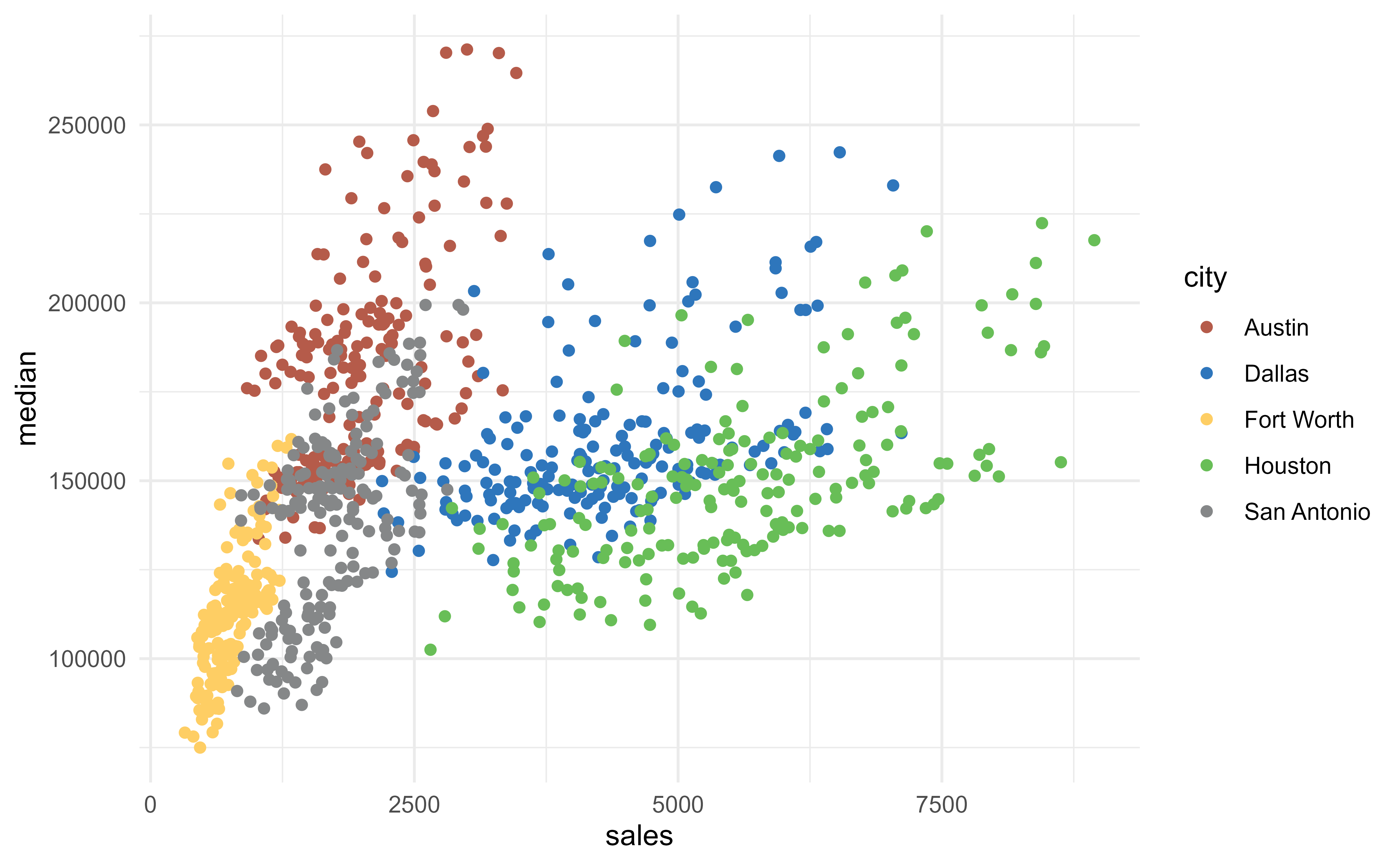
ggplot(txsamp, aes(x = sales, y = median)) +
  geom_point(aes(colour = city)) +
  scale_color_bde_d() +
  theme_minimal()



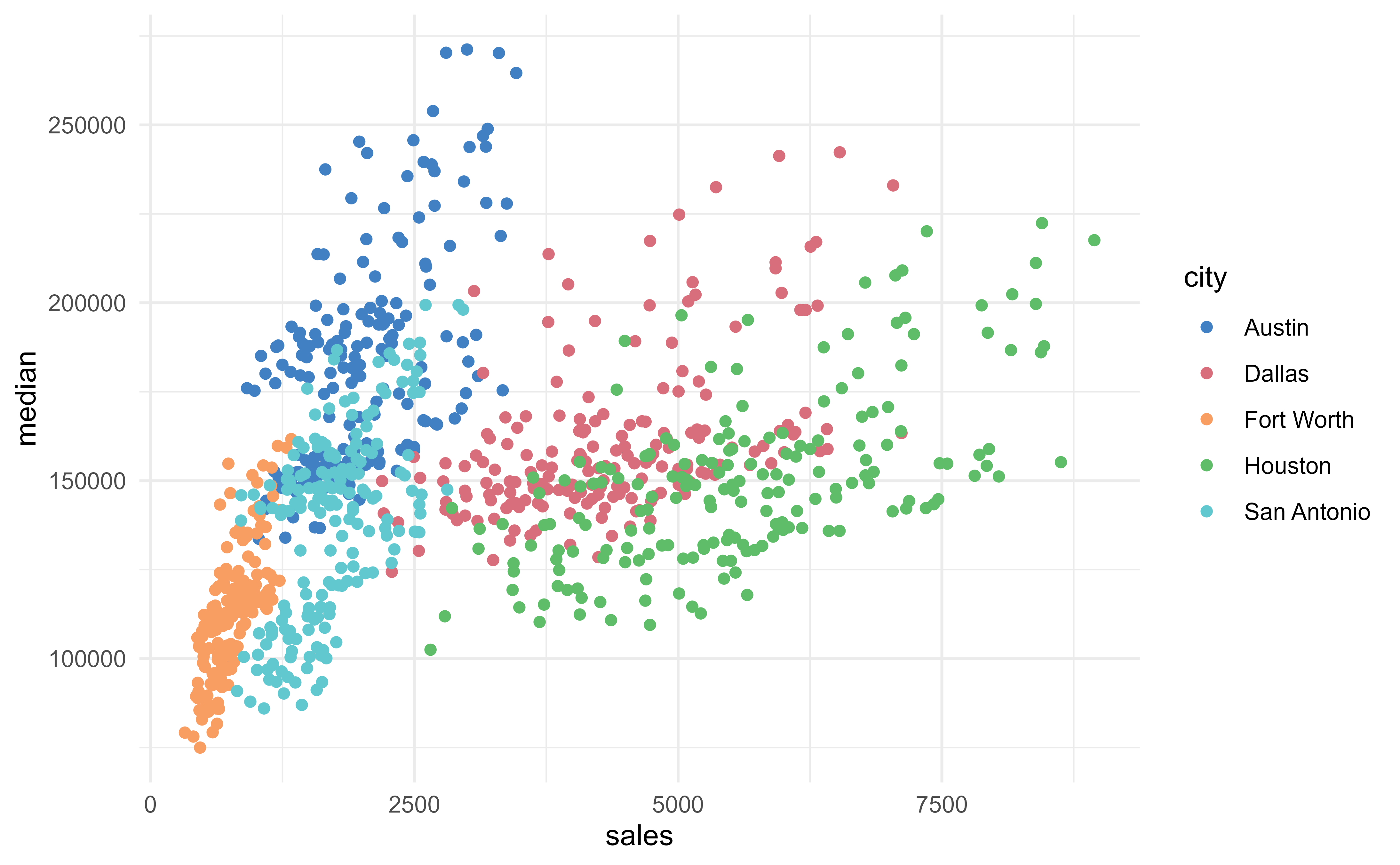ggplot(txsamp, aes(x = sales, y = median)) +
  geom_point(aes(colour = city)) +
  scale_color_bde_d("bde_rose_pal") +
  theme_minimal()