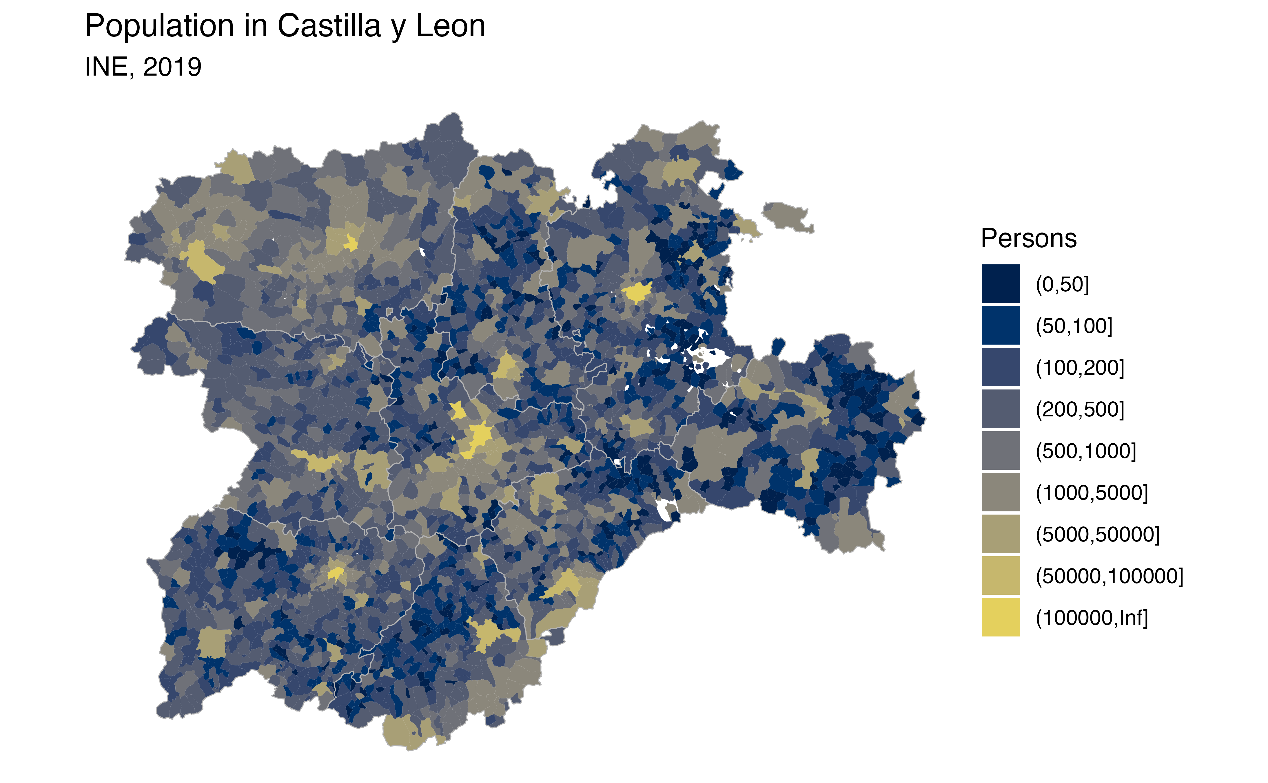
Get boundaries of municipalities in Spain.
Usage
esp_get_munic(
  year = 2024,
  epsg = 4258,
  cache = deprecated(),
  update_cache = FALSE,
  cache_dir = NULL,
  verbose = FALSE,
  region = NULL,
  munic = NULL,
  moveCAN = TRUE,
  ext = "gpkg"
)
Source
https://gisco-services.ec.europa.eu/distribution/v2/.
Copyright: https://ec.europa.eu/eurostat/web/gisco/geodata/statistical-units.
Arguments
- year
Year character string or number. Release year of the file. See
giscoR::gisco_get_lau()andgiscoR::gisco_get_communes()for valid values.- epsg
Character string or number. Projection of the map: 4-digit EPSG code. One of:
"4258": ETRS89."4326": WGS84."3035": ETRS89 / ETRS-LAEA."3857": Pseudo-Mercator.
- cache
![[Deprecated]](figures/lifecycle-deprecated.svg) . This argument is
deprecated, the dataset will always be downloaded to the
. This argument is
deprecated, the dataset will always be downloaded to the cache_dir.- update_cache
Logical. If
TRUE, refreshes the cached file and forces a new download. Defaults toFALSE.- cache_dir
Character string. A path to a cache directory. See Caching.
- verbose
A logical value. If
TRUEdisplays informational messages.- region
Optional. A vector of region names, NUTS or ISO codes (see
esp_dict_region_code()).- munic
Character string. A name or
regexexpression with the names of the required municipalities. UseNULLto return all municipalities.- moveCAN
A logical
TRUE/FALSEor a vector of coordinatesc(lat, lon). It places the Canary Islands close to Spain's mainland. Initial position can be adjusted using the vector of coordinates. See Displacing the Canary Islands inesp_move_can().- ext
Character. Extension of the file (default
"gpkg"). SeegiscoR::gisco_get_nuts().
Value
A sf object.
Details
When using region you can use and mix names and NUTS codes (levels 1, 2 or
3), ISO codes (corresponding to level 2 or 3) or "cpro"
(see esp_codelist).
When calling a higher level, such as a province, Autonomous Community, Autonomous City or NUTS 1 region, all municipalities of that level are added.
Note
Please check the download and usage provisions on
giscoR::gisco_attributions().
Caching
Functions that download data store files in cache_dir. When cache_dir
is NULL, they use the active package cache, which defaults to a temporary
directory. Set update_cache = TRUE to replace an existing cached file.
See Caching strategies in esp_set_cache_dir() to configure a
persistent cache.
See also
Municipality-level datasets:
esp_get_capimun(),
esp_get_munic_siane()
GISCO boundary data:
esp_get_ccaa(),
esp_get_nuts(),
esp_get_prov(),
esp_get_spain()
Examples
# \donttest{
# The Spanish Lapland:
# https://en.wikipedia.org/wiki/Celtiberian_Range

# Get municipalities.
spanish_laplad <- esp_get_munic(
  year = 2023,
  region = c(
    "Cuenca", "Teruel",
    "Zaragoza", "Guadalajara",
    "Soria", "Burgos",
    "La Rioja"
  )
)
#> ! The file to download is "61 Mb".

breaks <- sort(c(0, 5, 10, 50, 100, 200, 500, 1000, Inf))
spanish_laplad$dens_breaks <- cut(spanish_laplad$POP_DENS_2023, breaks,
  dig.lab = 20
)

cut_labs <- prettyNum(breaks, big.mark = " ")[-1]
cut_labs[length(breaks)] <- "> 1000"

library(ggplot2)
ggplot(spanish_laplad) +
  geom_sf(aes(fill = dens_breaks), color = "grey30", linewidth = 0.1) +
  scale_fill_manual(
    values = hcl.colors(length(breaks) - 1, "Spectral"), na.value = "black",
    name = "people per sq. kilometer",
    labels = cut_labs,
    guide = guide_legend(
      direction = "horizontal",
      nrow = 1
    )
  ) +
  theme_void() +
  labs(
    title = "The Spanish Lapland",
    caption = giscoR::gisco_attributions()
  ) +
  theme(
    text = element_text(colour = "white"),
    plot.background = element_rect(fill = "grey2"),
    plot.title = element_text(hjust = 0.5),
    plot.subtitle = element_text(hjust = 0.5, face = "bold"),
    plot.caption = element_text(
      color = "grey60", hjust = 0.5, vjust = 0,
      margin = margin(t = 5, b = 10)
    ),
    legend.position = "bottom",
    legend.title.position = "top",
    legend.text.position = "bottom",
    legend.key.height = unit(0.5, "lines"),
    legend.key.width = unit(1, "lines")
  )

# }
# }