Get started

CatastRoNav provides access to services from the Cadastre of Navarre. With CatastRoNav, you can retrieve addresses, buildings and cadastral parcels through its INSPIRE ATOM and WFS services. You can also download georeferenced images through its WMS service.

INSPIRE services

The INSPIRE Directive aims to create a European Union Spatial Data Infrastructure (SDI) for EU environmental policies and policies or activities that may affect the environment. This infrastructure enables public sector organizations to share environmental spatial information, facilitates public access to spatial information across Europe and assists in policy-making across boundaries.

Source: INSPIRE Knowledge Base.

The Cadastre of Navarre implements the INSPIRE Directive through three services:

1. ATOM service: Downloads complete municipal cadastral datasets.
2. WFS service: Retrieves cadastral features within a supplied bounding box.
3. WMS service: Downloads georeferenced map images for addresses, buildings and cadastral parcels.

ATOM download and WFS query functions return addresses, buildings and cadastral parcels as sf objects from the sf package. ATOM index and search functions return tibbles. WMS functions return georeferenced images as SpatRaster objects from the terra package. ATOM index reference timestamps use UTC. Municipal downloads return NULL if no municipality matches or the data cannot be downloaded. Errors when reading spatial files propagate to the caller. Municipality inputs must be a single name, partial name or cadastral code. Codes can be strings or numbers, such as "201" or 201. Empty inputs, NA and vectors produce an error before any network request.

Downloads are always cached, as in CatastRo. The ATOM cache argument is deprecated. Use a temporary cache_dir for session-only downloads and update_cache = TRUE to refresh ATOM or WMS data. Failed ATOM updates preserve previously cached files. WFS queries reuse cached responses until the cache is cleared with catrnav_clear_cache().

ATOM downloads and WFS queries share the catastronav_timeout and catastronav_ssl_verify options and the CATASTRONAV_TIMEOUT and CATASTRONAV_SSL_VERIFY environment variables. See catrnav_set_cache_dir() for configuration precedence and cache subdirectories.

Examples

Working with layers

This example demonstrates the main capabilities of CatastRoNav by recreating a cadastral map of the area around El Sadar Stadium. We use the WMS and WFS services to retrieve different layers.

# Retrieve buildings within a bounding box.
# Coordinates can be obtained from https://boundingbox.klokantech.com/.

library(CatastRoNav)
library(dplyr)
library(ggplot2)
library(mapSpain)
library(sf)

stadium <- catrnav_wfs_get_buildings_bbox(
  c(-1.6384926614, 42.7958160568, -1.6354170622, 42.7974640323),
  srs = 4326
)

# Transform to the WMS query CRS.

stadium_parcel_pr <- sf::st_transform(stadium, 3857)

# Extract parcel label imagery.

labs <- catrnav_wms_get_layer(
  stadium_parcel_pr,
  what = "parcel",
  srs = 3857
)

# Plot the layers.
library(tidyterra) # Plot SpatRaster layers.

ggplot() +
  geom_spatraster_rgb(data = labs) +
  geom_sf(data = stadium, fill = "red", alpha = .5) +
  coord_sf(crs = 25830)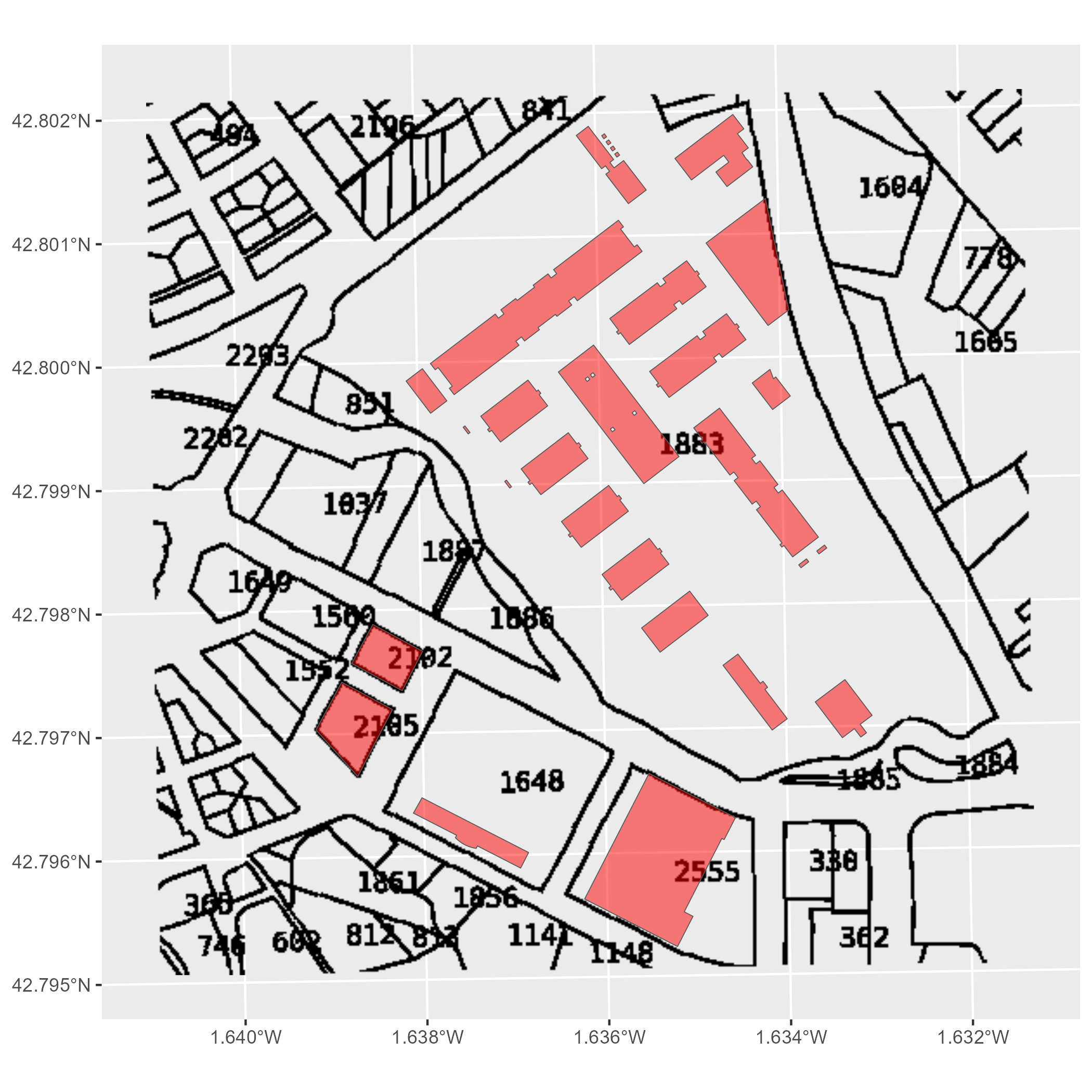

Figure 1: Cadastral layers around El Sadar Stadium

Thematic maps

We can also create thematic maps from attributes in spatial objects. This example visualizes urban growth in Pamplona with CatastRoNav, reproducing a map by Dominic RoyC) (Royé 2019).

First, we retrieve the geometry of Pamplona’s city center with mapSpain:

# Use mapSpain to obtain the city geometry.
pamp <- esp_get_capimun(munic = "^Pamplona")

# Transform to ETRS89 / UTM zone 30N and add a 1,250 m buffer.
pamp_buff <- pamp |>
  st_transform(25830) |>
  st_buffer(1250)

Next, we retrieve buildings using the WFS service:

pamp_bu <- catrnav_wfs_get_buildings_bbox(pamp_buff, count = 10000)

Then, we crop the buildings to the buffer created earlier:

# Crop buildings.

dataviz <- st_intersection(pamp_bu, pamp_buff)

ggplot(dataviz) +
  geom_sf()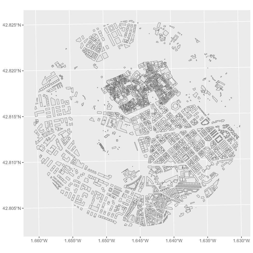

Figure 2: Buildings within the Pamplona buffer

Next, we extract the construction year from the beginning column:

# Extract the first four characters.
year <- substr(dataviz$beginning, 1, 4)

# Replace entries that do not look like years with "0000".
year[!(year %in% 0:2500)] <- "0000"

# Convert the years to integers.
year <- as.integer(year)

# Add a new column.
dataviz <- dataviz |>
  mutate(year = year)

Finally, we group the data by construction year and create the visualization. Here, cut() creates classes for each decade from 1900 onward:

dataviz <- dataviz |>
  mutate(
    year_cat = cut(year, breaks = c(0, seq(1900, 2030, by = 10)), dig.lab = 4)
  )

# Adjust the color palette.

dataviz_pal <- hcl.colors(length(levels(dataviz$year_cat)), "Spectral")

ggplot(dataviz) +
  geom_sf(aes(fill = year_cat), color = NA) +
  scale_fill_manual(values = dataviz_pal) +
  theme_void() +
  labs(title = "PAMPLONA", fill = "") +
  theme(
    panel.background = element_rect(fill = "black"),
    plot.background = element_rect(fill = "black"),
    legend.justification = .5,
    legend.text = element_text(
      colour = "white",
      size = 12
    ),
    plot.title = element_text(
      colour = "white", hjust = .5,
      margin = margin(t = 30),
      size = 30
    ),
    plot.caption = element_text(
      colour = "white",
      margin = margin(b = 20), hjust = .5
    ),
    plot.margin = margin(r = 40, l = 40)
  )

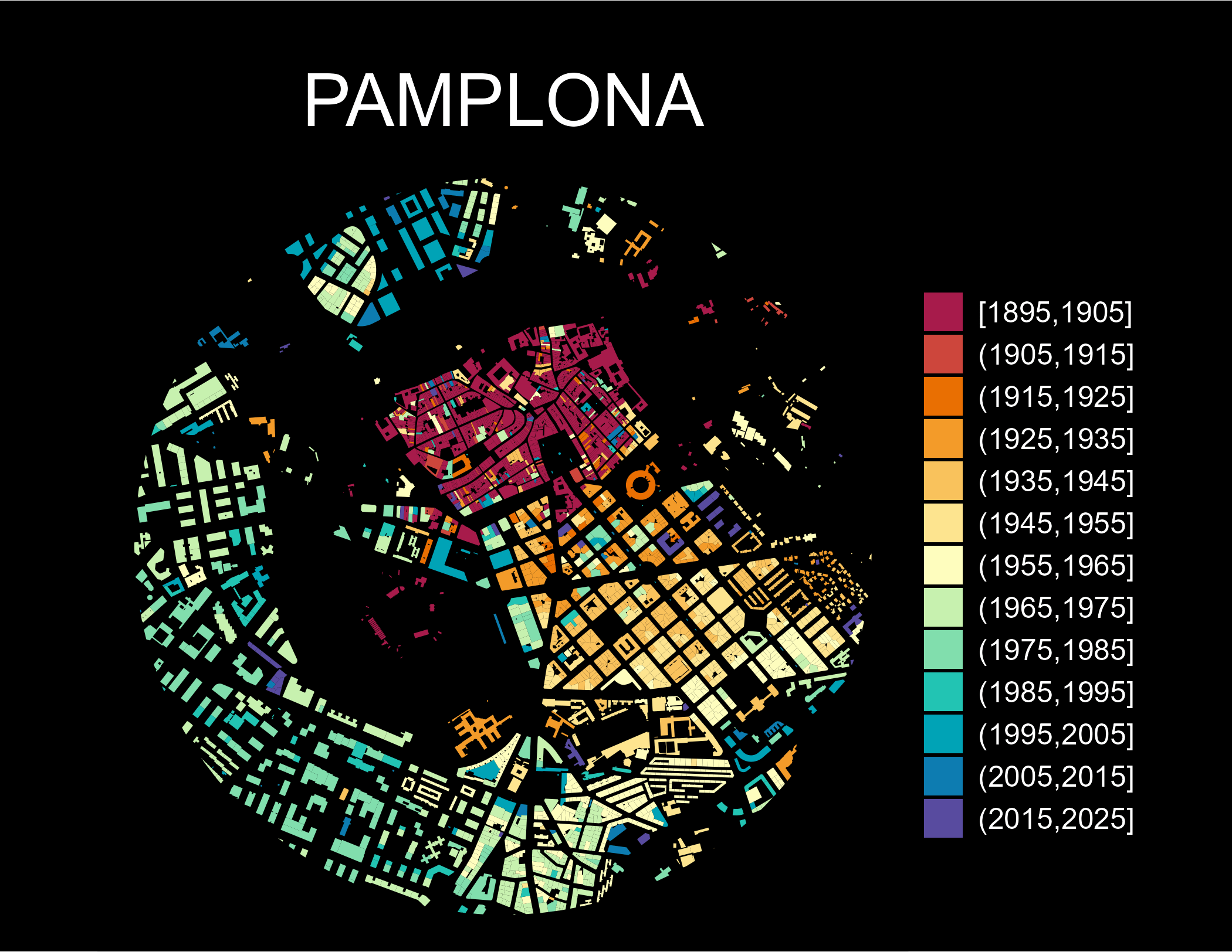
Figure 3: Urban growth in Pamplona

References

Royé, Dominic. 2019. Visualize Urban Growth. https://dominicroye.github.io/blog/visualize-urban-growth/.