
CatastRo provides access to services from the Spanish Cadastre. With CatastRo, you can retrieve addresses, buildings, cadastral parcels and georeferenced map images.
OVCCoordenadas service
The OVCCoordenadas service retrieves the coordinates of a known cadastral reference (geocoding). It can also retrieve cadastral references near a pair of coordinates (reverse geocoding). CatastRo returns the results as tibbles. These operations are described in detail in the corresponding vignette (see vignette("ovcservice", package = "CatastRo")).
INSPIRE services
The INSPIRE Directive aims to create a European Union Spatial Data Infrastructure (SDI) for the purposes of EU environmental policies and policies or activities which may have an impact on the environment. This European Spatial Data Infrastructure enables the sharing of environmental spatial information among public sector organizations, facilitates public access to spatial information across Europe and assists in policy-making across boundaries.
The Spanish Cadastre implementation of the INSPIRE Directive (see Spanish Cadastre INSPIRE services) provides access to spatial objects from the cadastral database:
-
Vector objects: Parcels, addresses, buildings, cadastral zones and more. CatastRo returns these as
sfobjects from the sf package. -
Imagery: Image layers representing the same information as the vector objects. CatastRo returns these as
SpatRasterobjects from the terra package.
These services cover 95% of the Spanish territory, excluding the Basque Country and Navarre1, which have their own independent cadastral offices.
There are three INSPIRE services:
ATOM service: The ATOM service downloads complete municipal datasets for different cadastral elements.
WFS service: The WFS service downloads vector objects for specific cadastral elements. Note that there are restrictions on the extent and number of elements that can be queried. For full municipal downloads, prefer the ATOM service.
WMS service: The WMS service downloads georeferenced map images for different cadastral elements.
Examples
Working with layers
This example demonstrates some of the main capabilities of the package by recreating a cadastral map of the surroundings of the Santiago Bernabéu Stadium. We use the WMS and WFS services to retrieve different layers.
# Extract buildings by bounding box.
# Check https://boundingbox.klokantech.com/

library(CatastRo)

stadium <- catr_wfs_get_buildings_bbox(
  c(-3.6891446916, 40.4523311971, -3.687462138, 40.4538643165),
  srs = 4326
)

# Extract cadastral parcels using a spatial object as the query input.

stadium_parcel <- catr_wfs_get_parcels_bbox(stadium)

# Transform to the tile CRS.

stadium_parcel_pr <- sf::st_transform(stadium_parcel, 25830)

# Extract parcel label imagery.

labs <- catr_wms_get_layer(
  stadium_parcel_pr,
  what = "parcel",
  styles = "BoundariesOnly",
  srs = 25830
)

# Plot.
library(ggplot2)
library(tidyterra) # Plot SpatRaster layers.

ggplot() +
  geom_spatraster_rgb(data = labs) +
  geom_sf(
    data = stadium_parcel_pr,
    fill = NA, col = "red", linewidth = 2
  ) +
  geom_sf(data = stadium, fill = "red", alpha = .5) +
  coord_sf(crs = 25830)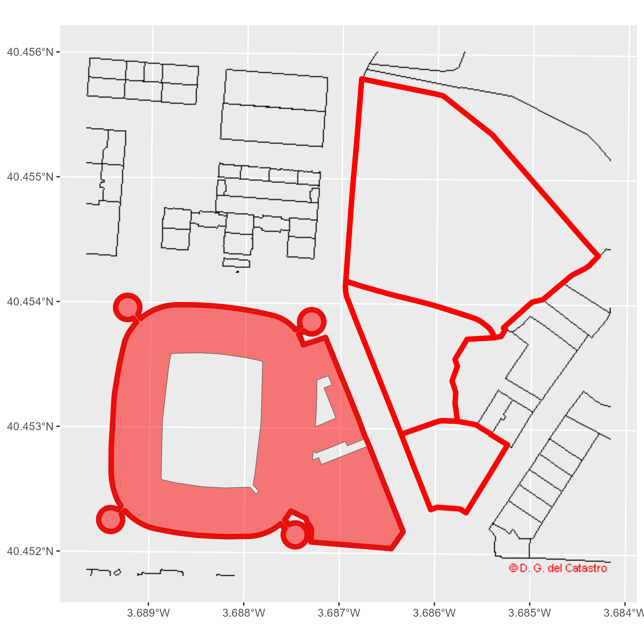
Figure 1: Santiago Bernabéu example
Thematic maps
We can also create thematic maps from attributes in the spatial objects. This example visualizes the urban growth of Granada with CatastRo, reproducing a map by Dominic Royé (Royé 2019) with the ATOM service.
First, we retrieve the geometry of Granada’s city center with mapSpain:
library(dplyr)
library(sf)
library(mapSpain)

# Use esp_get_capimun() to get the city geometry.

city <- esp_get_capimun(munic = "^Granada$")
Next, we use catr_get_code_from_coords() to identify Granada’s cadastral municipality code, then download its buildings with catr_atom_get_buildings().
city_catr_code <- catr_get_code_from_coords(city)

city_catr_code
#> # A tibble: 1 × 12
#>   munic   catr_to catr_munic catrcode cpro  cmun  inecode nm      cd    cmc   cp    cm
#>   <chr>   <chr>   <chr>      <chr>    <chr> <chr> <chr>   <chr>   <chr> <chr> <chr> <chr>
#> 1 GRANADA 18      900        18900    18    087   18087   GRANADA 18    900   18    87

city_bu <- catr_atom_get_buildings(city_catr_code$catrcode)
Next, we limit the analysis to a circle with a radius of 1.5 km around the city center:
buff <- city |>
  # Adjust CRS to 25830 for buildings.
  st_transform(st_crs(city_bu)) |>
  # Buffer.
  st_buffer(1500)

# Cut buildings.
dataviz <- st_intersection(city_bu, buff)

ggplot(dataviz) +
  geom_sf()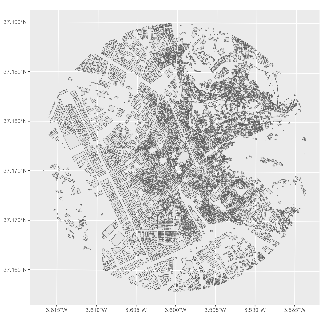
Figure 2: Minimal cadastral map of Granada
Next, we extract the construction year from the beginning column:
# Extract the first four characters.
year <- substr(dataviz$beginning, 1, 4)

# Replace entries that do not look like years with 0000.
year[!(year %in% 0:2500)] <- "0000"

# Convert to integers.
year <- as.integer(year)

# Add a new column.
dataviz <- dataviz |>
  mutate(year = year)
Finally, we group the data by construction year and create the visualization. The cut() function creates classes for each decade from 1900 onward:
dataviz <- dataviz |>
  mutate(
    year_cat = cut(year, breaks = c(0, seq(1900, 2030, by = 10)), dig.lab = 4)
  )

ggplot(dataviz) +
  geom_sf(aes(fill = year_cat), color = NA, na.rm = TRUE) +
  scale_fill_manual(
    values = hcl.colors(15, "Spectral"),
    na.translate = FALSE
  ) +
  theme_void() +
  labs(title = "GRANADA", fill = "") +
  theme(
    panel.background = element_rect(fill = "black"),
    plot.background = element_rect(fill = "black"),
    legend.justification = .5,
    legend.text = element_text(
      colour = "white",
      size = 12
    ),
    plot.title = element_text(
      colour = "white",
      hjust = .5,
      margin = margin(t = 30),
      size = 30
    ),
    plot.caption = element_text(
      colour = "white",
      margin = margin(b = 20),
      hjust = .5
    ),
    plot.margin = margin(r = 40, l = 40)
  )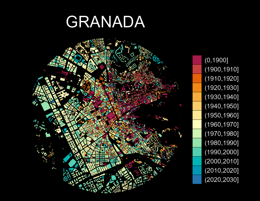
Figure 3: Granada - urban growth